ARC 3.5m | SPIcam
Last updated: Feb 23, 2016 - AB
Table of Contents
SPIcam is a general purpose, visible-wavelength, direct imaging CCD camera with > 50% QE between 400-900 nm, with a 6 position filter wheel. The detector in SPIcam is a backside-illuminated SITe TK2048E 2048x2048 pixel CCD with 24 micron pixels, giving an unbinned plate scale of 0.14 arc seconds per pixel and a field of view of 4.78 arc minutes square.
SPIcam is an acronym for Seaver Prototype Imaging camera; we would like to acknowledge the generous support of the Seaver Institute and the David and Lucille Packard Foundation who made construction of this instrument possible.
SPICAM has no internal reimaging optics, so the pixel scale is determined by the scale of the 3.5m F/10 telescope. This gives 0.14 arcsec/pixel. Since the seeing is significantly worse than this, the detector is almost always operated in binned mode, most commonly, 2x2 binning, giving 0.28 arcsec/pixel. Larger binning is certainly possible, leading to smaller images and reduced readout times.
The six position filter wheel in SPICAM takes 3" square filters. We have several filter wheels available; the most common filters used are either the SDSS u'g'r'i'z' filters or the MSSSO UBVRI filter set. Other filters are available, but require advance notice to get them loaded into a filter wheel. The full set of filters available at APO can be found here.
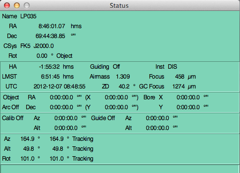
SPIcam is operated within the Telescope User Interface (TUI) software written and maintained by Russell Owen at the University of Washington. A detailed manual is available here. The main TUI status window looks like this:
2.2. Configuring the Instrument
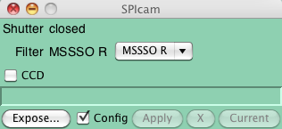
The instrument is configured using the SPIcam window accessible under the Inst menu from the main TUI window. This brings up the SPIcam control gui. Here we give brief overview of the SPIcam controls via the SPIcam control gui:
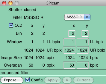
This window shows the current configuration (Shutter state, filter, binning, windowing, Image size, Overscan area). The configuration can be changed using the Show Config button; as with other TUI windows, the Apply button must be hit to implement any selected changes and all current selections are applied upon click.
Generally, the main item that is configured is changing the filter. The CCD binning is also configurable here, but is generally set to a value at the beginning of the night, and then left unchanged. This is done by clicking the CCD button in the config window. It will look like this:
Note that it is possible to write scripts to take sequences of exposures, e.g., changing filters between each exposure. The simplest scripts are just lists of low-level SPICAM commands, which are presented in Appendix D. More complex scripts with GUI interfaces can be written; see the TUI manual for more information.
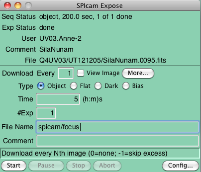
SPIcam exposures are taken using the Expose window which is opened using the Expose button in the SPIcam configuration window, the Expose gui looks like:
The expose window is in standard TUI format (for detailed description see here ), and, as for other instruments, shows status of the current exposure at the top, and allows you to set the object Type (for the FITS image header), exposure Time, number of Exposures, and root File Name. If you wish to add comments to the file header, place them in the Comments field.
All data will automatically be stored on arc-gateway under /export/images/<program ID>/<filename>. However, most users set TUI up to automatically transfer images to their local computer using the Preferences options in the main TUI window menu (see AutoGet and Save To options under Exposures). You can also define a subdirectory (TUI will even create it for you) by entering a name such as <subdir1>/<subdir2>/<filename> ;note, however, that a separate image number sequence will be started in each subdirectory.
The FITS header for each image stores the exposure time values (duration, start, stop) plus telescope parameters for future reference.
The Start button begins the exposure or exposure sequence.
- Start - This button starts the exposure or exposure sequence.
- Pause - This button pauses the exposure, you can start it again later.
- Stop - This button stops the exposure AND saves the current data to disk
- Abort - This button aborts an exposure. It DOES NOT save the data.
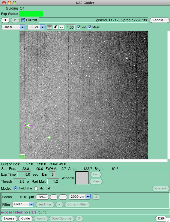
Guiding while using SPICAM is accomplished through use of the off-axis guider on the NA2 port.Control of the NA2 guide camera is obtained via the Guide selection in the main TUI window. This will open the following GUI:
To guide, find a star located in the guide camera image and guide on it via Field Star guiding. Manual guiding does not send guide corrections to the telescope, but just continues to take images.
You can guide on any object which is symmetric (galaxies with strong cores are fine), not too faint, and non-saturated. Optical double stars, late-type galaxies, and bipolar PNs may pose a problem for guiding, as will objects where you desire to observe a position away from the bright center (e.g., SNs near bright galaxies). Any object the guide software thinks is usable will be circled in green. If your favored guide object is not circled, it may be too faint, too bright, or too lumpy. If you really want to use an object that has no circle around it, try dragging a box around it to centroid it. If this succeeds (if a circle appears) then you are all set.
Use longer exposure times to get better signal from your star. The best exposure times are 5-30 seconds, but up to 120 seconds is usable if you can be patient. Longer exposure times can also help if you're having data transfer problems. Exposures shorter than about 3s are a waste of image-transfer bandwidth and may cause you to over-guide on seeing fluctuations. See more about guiding in Guiding with TUI User's Guide.
The telescope is focused by inspection of SPIcam images. Generally, focusing is most efficiently accomplished by letting the Observing Specialist focus the telescope. A focus script is available under the Scripts/SPICam/Focus TUI menu; this is what is used by the observing specialists to focus and provide a current seeing estimate.
As with all instruments, monitoring focus is advisable, as it will change over the course of the night, especially at the beginning of the night before the telescope has reached equilibrium.
Because SPICam is located on the NA2 image derotator, the chip can be oriented however the user prefers. At a Rot angle of 0, N is in the direction of increasing rows, and W in the direction of increasing columns.
The following table summarizes some of the chip characteristics; see more details in subsequent sections:
Number of rows Number of columns Pixel size Gain Readout noise Field of View 4.7 arcmin
Platescale Readout time is about 42 seconds in 2x2 binned mode.
3.2. Detector Layout/Cosmetics
The detector is cometically excellent.
3.3. Detector Linearity/Saturation
The CCD is linear up to ~64,000 counts, i.e. the full range of the A/D converter.
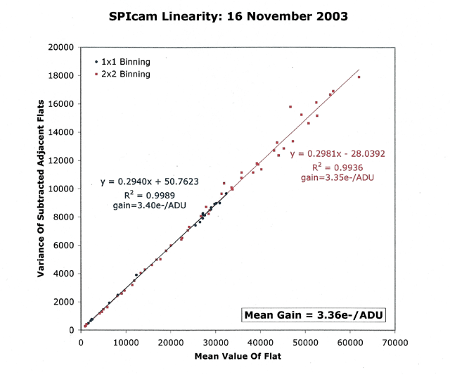
3.4. Detector Gain and Readout Noise
The gain has been measured to be 3.36 electrons/pixel, with a readout noise of 5.7 electrons/pixel.
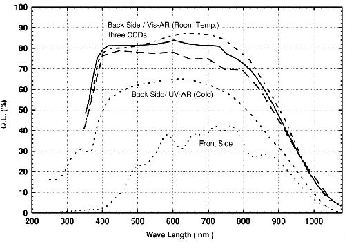
The following table shows the CCD quantum efficiency, as measured by SITe.
Wavelength (nm) QE (%) Notes 350 75.0 interpolated 400 84.0 measured 500 87.0 interpolated 550 87.2 measured 650 89.0 interpolated 700 87.4 measured 800 76.0 interpolated 900 49.3 measured 1000 17.0 interpolated
Exposure times can be estimated using the rough instrument zeropoints given in the following table (accurate only to 10-20 percent!), taken from an old compilation by Eugene Magnier, which gives coefficients for:
m = -2.5log(DN/sec) + C - K*(airmass - 1.0) + A*color i.e., a star of magnitude C will give 1 DN/sec if observed at low airmass.
filter lambda C K A color u' 3500A 21.38 0.48 x none g' 4700A 24.92 0.19 x none r' 6200A 24.93 0.11 x none i' 7700A 24.72 0.04 x none z' >8500A 23.43 0.06 x none U 3650A 22.10 0.44 -0.14 U-B B 4400A 24.43 0.25 0.04 B-V V 5500A 24.91 0.14 -0.02 B-V R 7000A x x x x I 9000A 24.53 0.06 0.04 V-I
The most important calibration for imaging are flat fields. Bias and dark frames may also be desireable. See the following sections for details.
4.1. Calibration Lamps and Control
There are bright and dim quartz lamps located on the truss at the top of the telescope that can be used for flat fields, taken off of the mirror covers. These are controlled by the Truss Lamps GUI under the Misc item in the command bar in the main TUI window. In contrast with many other TUI controls, these are turned on and off by simply hitting the On/Off buttons; there is no Apply button for these lamps.
Flat fields can be taken by shining the truss lamps onto closed primary mirror covers; no "white spot" is used at the 3.5m. Since the installation of improved baffling in the telescope, these "mirror cover" flats provide reasonable measurements of the variation in instrument/telescope response over the SPICAM field of view. Although twilight flats are still preferable and superflats taken from object images are best of all, mirror cover flats are a desirable alternative when the other kinds are not possible. Mirror cover flats will be slightly redder than the twilight sky or the night sky, and may therefore be more appropriate for photometry of red targets through broadband filters. Another issue is that long exposures are required for the bluest filters with the current calibration lamps.
Thanks to the new baffle, the illumination pattern of mirror cover flats now has very little dependence on rotator position, except in the outer corners of the image. Observers planning aperture photometry on small objects near the center of the field should not have to worry about rotator position for mirror cover flats. Observers doing surface photometry on larger objects or aperture photometry of multiple targets throughout the field may want to take flats at multiple rotator positions and combine them into a master flat. This does require coordination with the observing specialist, since we have to be very careful about having the mirror covers closed and motors active at the same time -- so be sure to communicate your plans clearly to the observing specialist.
Here are some suggested exposure times that should give 20K-30K counts. We do not have a current set of exposure suggestions for narrowband filters.
On Feb 9, 2012 the Bright and Dim Quartz truss lamps were upgraded on the telescope. This changed the recommended exposure times for flat fields. The times prior to this date are being retained in the table below for archiving purposes.
u' Brt Qtz (900s gives about 14K counts) (360s gives about 11K counts) g' Brt Qtz 5s 3s g' Dim Qtz 300s 30s r' Dim Qtz 90s 6s i' Dim Qtz 60s 3s z' Dim Qtz 90s 5s U Brt Qtz (360s gives about 15K counts) B Brt Qtz 20s 17s V Brt Qtz 3s 2s V Dim Qtz 250s 15s R Dim Qtz 75s 5s I Dim Qtz 30s 3s Hα Brt Qtz 10s
In a full frame or a subframe that extends to the right edge of the chip, a bad column appears a few columns before the overscan, with counts of 65.5K. At 1x1 binning the bad column is a single column; at 2x2 binning one neighboring column is affected as well. The counts remain a little bit above the regular bias level for two or three columns after the bad column.
For a subframe that doesn't extend to the right edge of the chip, the> bad column appears right at the beginning of the overscan and only peaks 10-15 counts above bias. The height of this peak is constant; no dependence on size or positioning of subframe (aside from 'not at the right edge of the chip'). At both 1x1 and 2x2 binning this appears as a single column.
A subframe at the bottom of the chip will have shorter readout time. A subframe at the top of the chip will have the same readout time as a full frame. This is because the rows below the subframe get read out at normal > speed and then thrown away; the rows above the subframe get thrown away without being read. The same thing is happening in the serial read direction, left-right; the columns to the left of the subframe are read and the columns to the right are skipped. The left-right positioning has little effect on the readout time because the serial reads are faster than the parallel reads, but the same principle applies.
The overscan is over on the right side of the image and in order to "read" non-physical pixels, it needs to be beyond the right edge of the chip. So it seems that in the process of skipping the columns after the subframe and before the edge of the chip, the readout process is probably including just one physical column before the true overscan. That physical column is affected by the charge from the nearby bad column, so it's a little bit above bias.
Be sure to turn off any calibration lamps you may have used, then hand over the instrument by simply quitting out of the SPIcam instrument control window in TUI. In some circumstances, you may continue to use the instrument after your shift, e.g., you are the first half observer and the scheduled second-half observer is not using the SPIcam. Ask your Observing Specialist for permission to do so if circumstances warrant.
6.1. Data Storage and Retrieval
Your data will remain on arc-gateway.apo.nmsu.edu:/export/images/your program code/UTYYMMDD/ for 9 to 12 months before being automatically deleted. Data can be accessed via scp or sftp to the institutions' observer accounts on arc-gateway (you can also use ftp and the images account and password); call APO (575-437-6822) if you are unsure of the correct login.
See also the SPIcam Data Reduction guide.
Please find additional information for taking and reducing data here.
A. Instrument Design
See the SPIcam commissioning report.
Typical data: bias, flat, darks
D. Basic low-level commands (for scripting)
spicam filter 1|2|3|4|5|6 : sets filter to specified position
spicamExpose object|flat|dark|bias time=time [n=nexp] [name=root] : takes specified type of exposure, with specified exposure time, [number of exposures], [root file name]
Examples:
spicam filter 1 #(this command will change the filter wheel to filter position 1)
spicamExpose object time=10 n=1 name=spicam_exposure #(this command will take 1 object image of time 10s with the name spicam_exposure.fits) If making a Run_Command script TUI knows to wait for commands to be executed before continuing so listing one command after another is acceptable.
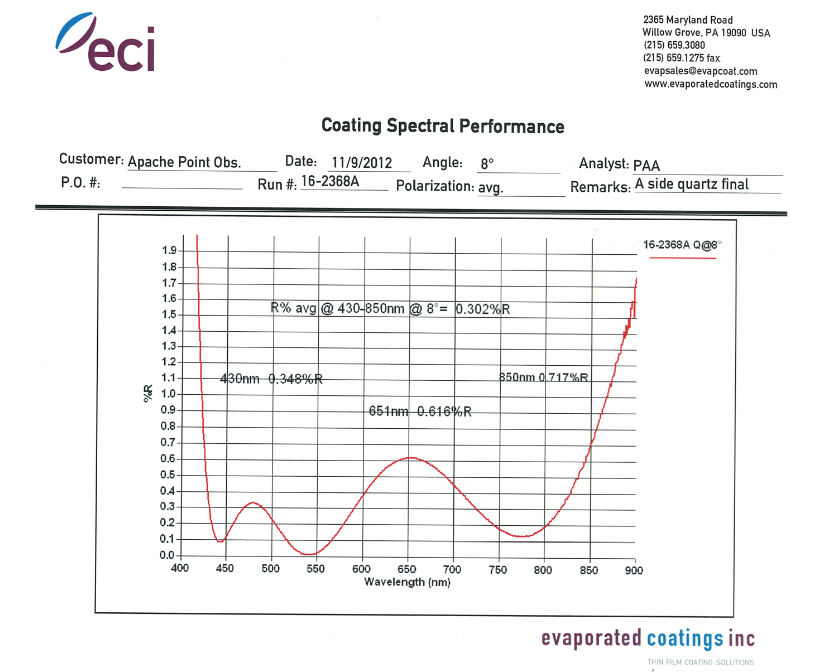
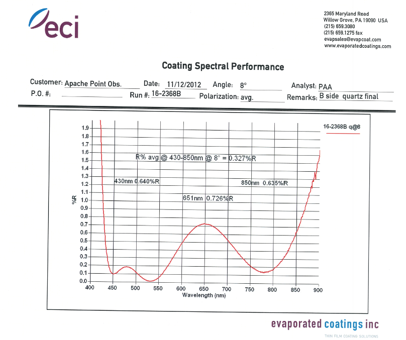
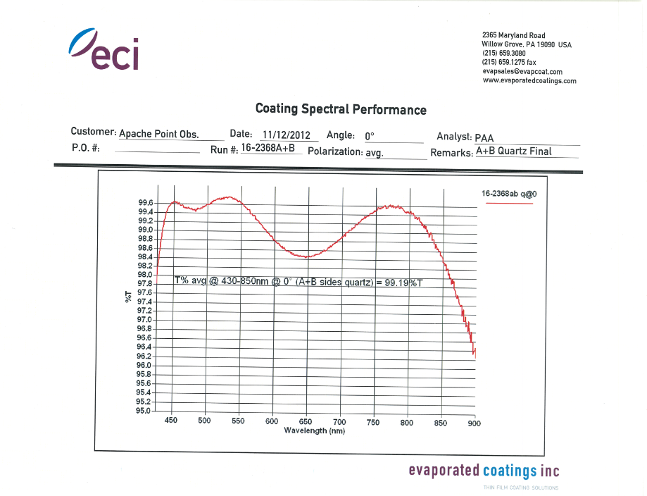
The following plots show reflectivity of AR coatings on both sides of the instrument window and combined transmission for the entire window (last image). These are as of 12/5/12.