ARC 3.5m | GIFS (DRP)
Last updated: September 16, 2014 - AW
1. Data Reduction Requirements1. Data Reduction Requirements
2. Calibration Data Requirements
3. "Standard" Calibrations
3.1. Bias Subtraction
3.2. Flat Fielding
4. Reducing Your Data
4.1. Direct Imaging Data
4.2. IFS Acquisition Mode Data
4.3. IFS Spectral Data
Questions?
2. Calibration Data RequirementsThe Goddard Integral Field Spectrograph Data Reduction Pipeline (GIFS DRP) and supplementary codes are written entirely in IDL. The source code, reference data, and sample data may be downloaded by clicking this link. Beyond the bias-subtracting and flat-fielding procedure defined in Section 3, this documentation and pipeline are useful only for the IFS mode of the instrument (with the lenslet array in place); filter imaging data can be reduced using observers' method(s) of choice.
System Requirements:
- IDL v8 or higher
- most up-to-date version of the pipeline, stored in your IDL path (LAST UPDATE: SEPTEMBER 5, 2014)
- The IDL Astronomy User's Library
- A three-button mouse (on Macs, can be activated in X11 preferences)
That's it! No working knowledge of IDL is necessary, though it may be helpful; any heavy lifting by the user is done through a GUI.
3. "Standard" CalibrationsAt present, the GIFS DRP only handles the complex task of translating to usable data cubes from raw IFS data. It does not perform flat-fielding or bias subtraction, though we list in the next section some recommendations on those tasks. Take flats (in direct imaging mode) and bias frames as directed in the GIFS Handbook.
For the GIFS DRP specifically, observers need to take two additional non-standard data frames each night: for each grating/filter used: an IFS dispersed frame with the Helium, Neon, and Argon truss lamps (not either of the Quartz lamps), which we'll call HENEAR, and one IFS acquisition frame (no disperser in place) with the Bright Quartz lamp on, which we'll call BRQRTZ. In addition, the team takes calibration data roughly once per year to build new reference files -- available in the above DRP download -- which are used in the reduction process. There are four reference files associated with each grating, plus one for acquisition mode, which are described in Table 1.
Table 1: Reference Files (provided in download) File Name Contents File Nickname acquisition_grid.fits Location of lenslets across detector without disperser in place REF_ACQ_GRID GRATINGNAME_grid.fits Location of lenslets across detector with disperser in place REF_GRID GRATINGNAME_trace.fits Spectral dispersion information TRACE GRATINGNAME_distortion.fits Spectral Distortion information DISTORTION GRATINGNAME_wave.fits Wavelength solution WAVE
Table 2: GIFS Data (taken by user) Image Contents File Nickname IFS image with Bright Quartz lamp on (i.e. no disperser in place) BRQRTZ IFS spectral image with Helium, Neon, and Argon lamps on HENEAR IFS spectral image with Bright Quartz, Helium, Neon, and Argon lamps on BRQRTZ_HENEAR Science target in IFS acquisition mode (i.e. no disperser in place) ACQ Science target in IFS spectral mode SCIENCE
3.1 Bias SubtractionThis step should be performed before starting the GIFS DRP routines. As noted in the instrument handbook, a non-repeatable striping is found in most bias frames. In September 2014, this was thought to be a ground loop in the instrument, similar to the one seen in DIS. The GIFS team will work towards fixing it at the end of this month.
3.2 Flat Fielding4. Reducing Your DataWe recommend the observer obtain flat-field calibration data using the BrQz lamps in order to correct pixel-to-pixel sensitivity variations.
Once the direct imaging data have been bias-subtracted and flat-fielded, they are ready for scientific analysis.
4.2 IFS Acquisition Mode DataData taken in the IFS acquisition mode, that is, when the IFS optics (the lenslet array, bare or pinhole mask) are in place, but the light is not dispersed, can aid in understanding the position of your science target on the detector before dispersion. We refer to your acquisition-mode image as ACQ. The two steps to producing an acquisition-mode image are: (1)Refine the lenslet grid location, and (2)Extract Science Image. These steps are explained in more detail below.
Refining Lenslet Grid Location
- Make sure the pipeline code is in your IDL path (Not sure how to do that? Here are some helpful suggestions.). Open up a terminal and navigate to the directory where your data (ACQ and BRQRTZ) live.
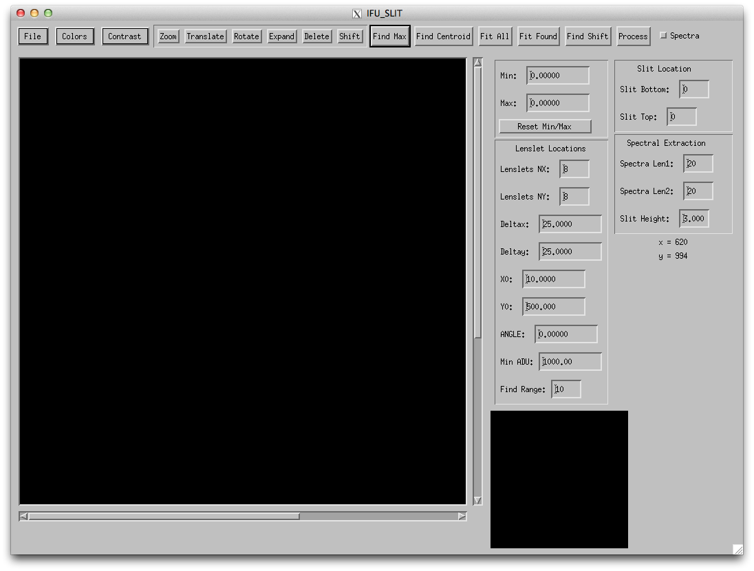
- Start up IDL and type "ifu_slit" at the prompt. This will open up a GUI (may take a few moments). At first, the image window will be empty (see Figure 1).
- Read in your BRQRTZ frame by going to File>>Read Image and selecting the correct file (see Figure 1).
Figure 1: IFU_SLIT GUI
- Read in the reference acquisition-mode grid by going to File>>Read Grid and selecting the REF_ACQ_GRID.
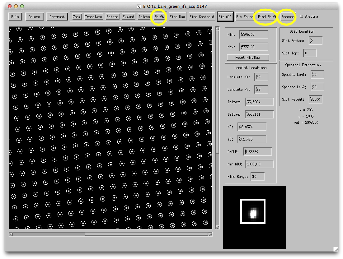
- Use the "Shift" button to fine tune the location of the circles (representing the lenslets) so that they best line up with the spots. You may not need to do much here. DO NOT use the "Translate" button for this task. When satisfied, press "Find Shift," then "Fit Found." See Figure 2 for an example of what you should see and what buttons to use.
Figure 2: Shifting the Lenslet Grid
- Save your new grid positions by going to File>>Write Grid. The program will offer a name that's just yourBRQRTZfilename_grid.fits which you can either keep or change. We'll refer to this new grid file as NEW_ACQ_GRID
- You'll continue to use this GUI in the next section, but if you wish, exit the GUI by going to File>>Exit.
Extract Science Image
- If neccesary, re-start ifu_slit from the IDL command line.
- Read in your ACQ frame by going to File>>Read Image and selecting the correct file.
- If you re-started the ifu_slit GUI, read in the new grid by going to File>>Read Grid and selecting the NEW_ACQ_GRID.
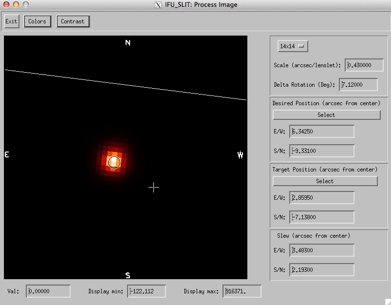
- Press the "process" button to process the results. A new GUI will pop up (see Figure 3. You can look at statistics and variations on the display, and you can also use this GUI to adjust the position of your target in real time using the "Desired Position," "Target Position," and "Slew" boxes on the right side of the GUI:
- By default, the desired position is set to the center of the array; if you would like your target elsewhere, press "Select" in the "Desired Position" box, and then click in the image where you'd like your target to be. A plus sign will mark the spot you chose, as shown in Figure 3.
- Mark the actual position of your target by first pressing "Select" in the "Target Position" box, and then clicking on the center of your target in the image. A circle will mark the target position.
- Use the output values in the "Slew" box in the offset window back in TUI to adjust your positioning.
Figure 3: Shifting the Lenslet Grid
- When finished, exit the GUI by pressing "Exit." A dialog box will automatically pop up, allowing you to save the final image as "yourACQfilename_results.fits," or whatever you choose.
- Exit the main GUI by going to File>>Exit
4.3 IFS Spectral Data5. Sample Data
Figure 4: GIFS DRP Flowchart
We outline the procedure for both building the reference files (done by the team) and reducing the science data in a flowchart in Figure 3. While we will not go into the details here for building the reference files, the code is all available (and commented) in the GIFS DRP download, and you are free to test it out yourself and contact the team if you have questions. As for reducing your IFS science data, we will describe the several steps to do so here. There are three general steps to reducing your data: first, you must refine the location of the lenslets on the detector, as that can shift slightly night to night, and even pointing to pointing (this also defines a zero point for your wavelength solution) using a dispersed IFS frame of the dome's truss lamps. Next, you'll apply the new lenslet grid to your science frame (dispersed) to extract the spectra. Finally, you'll put the extracted spectra into a standard wavelength cube and append a wavelength solution to the file. These basic steps are described in more detail below. We use the naming convention as listed in Table 1 and Table 2 to denote the difference data frames and reference files.
Refining Lenslet Grid Location
- Make sure the pipeline code is in your IDL path. You can find some helpful suggestions here.
- Open up a terminal or IDLDE and navigate to the directory where your data (SCIENCE, HENEAR_BRQRTZ, and HENEAR) are located.
- Start up IDL and type "ifu_slit" at the prompt. This will open up a GUI (may take a few moments). At first, the image window will be empty (see Figure 1).
- Read in your HENEAR frame by going to File>>Read Frame and selecting the correct file (see Figure 1).
- Clicking the "Colors" button will open a drop-down menu of image color scheme options.
- Clicking the "Contrast" button will open a drop-down menu of image scaling options.
Figure 5: IFU_SLIT GUI
- Read in the initial grid by going to File>>Read Grid and selecting the REF_GRID. This will also change the values of "Spectra Len1" and "Spectra Len2" on the right-hand side of the GUI, which will become important later.
- Read in the spectral dispersion file by going to File>>Read Spectral Trace File and selecting the TRACE file.
- Use the "Shift" button to fine tune the location of the circles (representing apertures to fit the lenslets positions) such that they best line up with the bright spots, as shown in Figure 6. The REF_GRID file may provide a good match to your data, which would then require no additional shifting of the apertures. DO NOT use the "Translate" button for this task.
- Make sure you are fitting to the correct spots! Use the images in Figure 6 for a guide.
- Unsure if you're using the right spot? Once you've set the grid, read in your BRQRTZ_HENEAR frame by going to File>>Read Image and selecting the correct file. Press the checkbox next to "Spectra" in the top right corner of the GUI, and confirm that the red lines (representing the spectral slit) roughly extend across the spectra.
- When satisfied with the grid locations on the HENEAR_BRQRTZ image, press "Find Shift," then "Fit Found," noting that the program may lag briefly after both while the fitting is taking place. See Figure 2 for an example of what should be visible and which buttons to use.
Figure 6: Shifting the Lenslet Grid Placing the grid for the red grating. Placing the grid for the greeting grating.
- Press the checkbox next to "Spectra" in the top right corner of the GUI. Now red lines representing the spectral slit will replace the white circles representing the lenslets.
- Press the "Process" button to process the results. Another GUI will pop up that presents cuts of the spectral cube you just created, which should have lines where the Helium, Neon, and Argon lamps emit. You can explore the cube with this GUI if you'd like. Once finished, exit the GUI; a save dialog which is set to save the data as "yourHENEARframename_spectra.fits." Change the name if you like, and save the file. We'll call this file NEW_REF_SPECTRA. This contains not only the spectral cube just created from the HENEAR data, but also the TRACE information, the shifted grid positions you created, and the spectral length parameters ("Len1" and "Len2").
Figure 8: IFU_SLIT: Processing Spectra
- You'll continue to use this GUI in the next section, but if you wish, exit the GUI by going to File>>Exit.
Build Science Spectra
- Re-start ifu_slit GUI from the IDL command line by typing ifu_slit.
- Read in your SCIENCE frame by going to File>>Read Frame and selecting the correct file.
- If you started up a new ifu_slit session (rather than continuing on from the "Refining Lenslet Grid Location" section), read in the new grid by going to File>>Read Grid and selecting the NEW_REF_SPECTRA.
- Also if you started up a new ifu_slit session, read in the spectral trace file by going to File>>Read Spectral Trace and selecting the NEW_REF_SPECTRA file.
- Check the box that says "Spectra" at the end of the top row. Now you have rectangular spectral extraction zones defined by a red line that is best seen in the magnification box at bottom right in the GUI. See Figure 3 for what the spectral extraction traces look like on top of a sample observation of a star.
Figure 8: Spectral Mode
- Press the "Process" button to process the results. The processed spectra GUI will pop up, showing the cuts of your science data spectral cube. You can look at statistics and variations on the display (perhaps more interesting to the average user here than with the reference cube), and when finished, Once finished, exit the GUI; a save dialog which is set to save the data as "yourSCIENCEframename_spectra.fits." Change the name if you like, and save the file. We'll call this file SCIENCE_SPECTRA.
- Exit the GUI by going to File>>Exit.
Build Science Data Cube
- From the IDL prompt, type "ifu_final_cube".
- You will immediately be prompted to enter a file name in a series of three windows, shown in Figure 4. First, you'll put in the SCIENCE_SPECTRA file (notice that the top of the window says "Input spectra file"). Once you press "OK," a second window will pop up, into which you'll put in the DISTORTION file (notice that the top of the window says "Input distortion file"). Once you press "OK," a third and final window will pop up, into which you'll put in the WAVE file (notice that the top of the window says "Input wave file").
Figure 9: Input Files for IFU_FINAL_CUBE
- Another helpful, but not required, GUI will pop up to allow you some examination of the spectral cube with the spectral distortion correction taken into account. Once you quit this GUI, the program will automatically save a "_cube.fits" file in your working directory.
The final "_cube.fits" file has two extensions: one with the data cube, and one with the wavelength solution. The data cube has 32x32 spatial elements, and approximately 300 elements in the wavelength range (exact number depends on the grating you use). You are now able to analyze the data using your favorite 3-dimensional visualization software.
Questions?
The GIFS-DRP was originally written by Don Lindler and has been modified for general use and is currently maintained by Ashlee Wilkins, a graduate student at the University of Maryland. Any questions/comments regarding the GIFS DRP should be directed to the GIFS team.