ARC 3.5m | DIS
Last updated: Feb 23, 2016 - AB
Table of Contents
DIS (Dual Imaging Spectrograph) is a medium dispersion spectrograph (resolving power 1000-7000) with separate red and blue channels. It was built at Princeton by Jim Gunn and collaborators and was upgraded (with new cameras/detectors/electronics) by Jeff Morgan and Peter Doherty at University of Washington (see Appendix B for instrument history). It can be also be used in imaging mode, although this is rarely done.
The optical path consists of a slit-mask assembly, a shutter, a dichroic with a transition wavelength around 5350 Angstroms, and two independent collimators and cameras for the blue and red sides. There is a grating turret that has 3 positions: one has permanently mounted mirrors in each channel for the imaging mode, while the other two each have a pair of grating mounts (one for each channel). The two CCDs the instrument currently uses are a Marconi CCD42-20-0-310 on the blue side, and an E2V CCD42-20-1-D21 on the red side.
In imaging mode, the field is limited by the slit mask assembly, giving a field of view of 4.36 arcmin with broadband filters and 4.0 arcmin with narrowband filters. In this mode, only a fraction of the detector is illuminated. The spatial scale in the blue channel is 0.40"/pixel; in the red channel, it is 0.42"/pixel.
There is an internal filter slot in each channel; a Gunn g filter can be placed in the blue channel, and a Gunn r filter in the red channel (for spectroscopic mode, these should generally be taken out of the beam). Some users have put 2-inch square filters into the slit wheel assembly; a few adapters may be available for this purpose. Note that since the slit wheel comes before the dichroic in the optical path, putting a filter here would likely restrict operation to just one channel.
For general purpose imaging, SPICAM is probably preferred over DIS due to its slightly better image quality and availability of a larger set of filters.
In spectroscopic mode, the spatial scales are 0.40"/pixel and 0.42"/pixel in the red and blue channels, respectively.
1.2.1 Gratings and Wavelengths
The following table lists the available gratings for DIS. Gratings should be referred to by the names in the leftmost column (e.g., B300, B400, etc.); the historical names for some of the older gratings are given in parentheses, but their use is deprecated.
Catalog Info
Catalog Info Standard DIS III grating setup is either
B400/R300 or B1200/R1200.Two pairs of gratings can be mounted in the turret at any time. The turret can be rotated from one position to another in about a minute; however, the positioning is not perfectly repeatable so it may be necessary to retake calibration exposures if the turret is rotated.
The gratings can be tilted in their housings to adjust the wavelength centers. For the lower resolution gratings (B400, B300, R300, R150, R300H), the entire wavelength range, from atmospheric cutoff to dichroic split in the blue, or from dichroic split to detector cutoff in the red, fits on the detector, so there is no need to adjust the center. For B1200, R830, and R1200, the desired wavelength center can be set via the tilt. There is some vignetting towards the chip edges, so it is advisable to set the wavelength center such that the target wavelengths are located towards the center of the chip, if possible. The tilts appear to be quite stable once set and typically do not move during turret rotation. Grating swaps can be made by observing specialists but take approximately 20 minutes; as a result, these are strongly discouraged during the night.
Your choice of gratings to be mounted, along with desired wavelength centers, should be specified in your observing proposal and explicitly be confirmed by email with the observing specalists (obs-spec at apo.nmsu.edu) several days prior to your observing time.
In both blue and red channels, spectra run horizontally along rows. In blue channel, wavelength increases with column number; in red channel wavelength decreases with column number.
The slit-mask assembly has 5 positions. For long slits, the slit length is 6 arcminutes. The standard setup has one open slot, plus long slits with widths corresponding to 0.9", 1.2" (with 2.0" occulting bar), 1.5", and 5.0"; these are all steel slits. The slit wheel can be commanded to rotate from one position to another in several seconds, so multiple slits could be used in a given night (although calibration data might need to be obtained for each slit).
The long slits are mounted in tilted positions in the slit wheel and their surfaces are aluminized to allow viewing of the field via the slit viewing camera; this is used for acquisition and guiding.
Slits available:
| Width (arcsec) | Location | Material |
0.9 |
DIS |
Steel |
1.2 (2" bar) |
3.5m Storage |
Steel |
1.5 |
DIS |
Steel |
2.0 |
3.5m Storage |
Steel |
5.0 |
3.5m Storage |
Steel |
5.0 |
DIS |
Precision width Si+Al |
20.0 |
3.5m Storage |
Precision width Si+Al |
Pinholes |
DIS |
Aluminum |
NOTES: The default wheel also contains one open position for imaging-mode observations.
Some users have constructed slit masks with multiple slits or slitlets that can be placed in the slit wheel. However, to keep all of the slits or slitlets in focus requires that these slit masks be placed flat in the slit wheel. There are spare slit wheels that allow for masks to be mounted flat. However, in this case, the slit viewing camera cannot be used, and users are required to acquire their field using the imaging mode in DIS. Anyone wishing to use DIS in this mode needs to carefully consider how to optimally make the slit masks and operate the instrument.
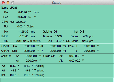
DIS is operated within the Telescope User Interface (TUI) software written and maintained by Russell Owen at the University of Washington. A detailed manual is available here. The main TUI status window looks like this:
2.2. Configuring the Instrument
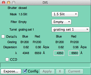
The instrument is configured using the DIS window accessible under the Inst menu from the main TUI window. This brings up the DIS instrument gui. Here we give brief overview of the DIS controls via the DIS instrument gui.
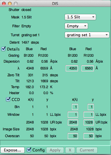
This window shows the current configuration (slit selection, grating selection, grating tilt/wavelength center, and CCD parameters. More details are available via the Details and CCD check boxes, and the configuration can be changed using the Config check box. As with other TUI windows, the Apply button must be hit to implement any selected changes and all current selections are applied upon click.
If you have informed the observing specialists of your setup in advance, the correct gratings and wavelength centers should be already set up. Of course, it is prudent for you to confirm these! Note that the wavelength centers only need to be correct to within a few Angstroms.
It is possible to change CCD windowing and binning in the DIS window by checking the CCD box. The CCD can be independently binned in either direction to change either the spatial scale, the dispersion (Å/pixel), or both. Binning might be advantageous if working in a readout noise limited regime where degradation of either spatial or spectral resolution is acceptable. With a slit length of 6 arcminutes, there are some unilluminated rows, so the file size can be reduced a bit by windowing the chip; you can window from (1:2048,101:950) without losing any data.
With a slit length of 6 arcminutes, there are some unilluminated rows, so the file size can be reduced a bit by windowing the chip. About 850 rows are illuminated but the exact location of the illuminated rows can change with grating alignment; if you want to window the chip, you should take a test exposure to determine the appropriate window.
DIS exposures are taken using the Expose gui, which is opened using the Expose button in the DIS instrument gui. The Expose gui looks like this:
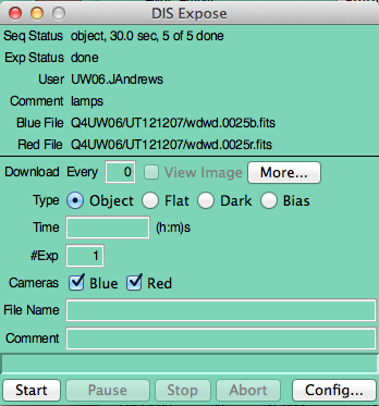
The Expose window is in standard TUI format (for detailed description see here ). It shows status of the current exposure at the top, and allows you to set the object Type (for the FITS image header), exposure Time, number of Exposures, and root File Name. If you wish to add comments to the file header, place them in the Comments field.
All data will automatically be stored on a local computer named arc-gateway in /export/images/<program ID>/<filename>. This can be accessed with a school specific username, for example, uwobserver. The passwords for these usernames change quarterly, and can be obtained by calling APO directly. However, most users set TUI up to automatically transfer images to their local computer using the Preferences options in the main TUI menu (see AutoGet and Save To options under Exposures). You can also define a subdirectory (TUI will even create it for you) by entering a name such as <subdir1>/<subdir2>/<filename>; note, however, that a separate image number sequence will be started in each subdirectory.
The FITS header for each image stores the exposure time values (duration, start, stop) plus telescope parameters for future reference.
The Start button begins the exposure or exposure sequence.
- Start - This button starts the exposure or exposure sequence.
- Pause - This button pauses the exposure, you can start it again later.
- Stop - This button stops the exposure AND saves the current data to disk
- Abort - This button aborts an exposure. It DOES NOT save the data.
Users should be aware that it is possible to write command scripts with sequences of commands. This can be done either by writing Python scripts for execution by TUI (see TUI documentation), or by writing lists of instrument level commands that can be run from the Run Commands window. This window is in the TUI menu under Scripts. Users can either type in the commands in that window, or read them from an input file. A list of useful instrument level commands is given in Appendix C .
2.4. The DIS Slitviewer Camera
There is an internal slitviewing camera in DIS that is used for target acquisition and guiding. The slitviewer camera is an E2V CCD47-10 thinned back-side illuminated CCD that is operated in an Andor-Apogee Aspen CG47 camera. The pixel size corresponds to 0.162 arcsec/pixel, giving a field of view of about 2.7 arcminutes on a side. Readout time is about 14s. Note that the slitviewer FOV is smaller than the DIS slit length, so you will not see the entire region over which you will be obtaining spectra.
Slitviewer Camera Summary:
- Camera manufacturer Apogee AP7
- CCD is a SITe SI-502A 512 x 512 back illuminated CCD
- CCD pixel size = 13 µm
- CCD gain = 4.5 e-/ADU
- CCD read noise = 7-11 e- / pixel
- Quantum Efficiency ~85% @ 680nm
- Dark Current: 1 e- / second
- Pixel scale = 0.162"/pixel binned 1x1
- Full well depth: 350k e-
- Saturation at 85K
- Installed filters (User selectable): N/A
- Available gratings (Observing Specialist installable): N/A
- Grating resolution: N/A
- Spectral Coverage: N/A
- Field of View: 165.9" x 165.9"
- Minimum Exposure: 0.01s
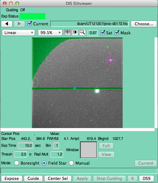
Control of the slitviewer is obtained via the DIS Slitviewer window accessible under the Guide selection in the main TUI menu. The slitviewer gui looks like this:
Images are obtained by setting an exposure time and hitting the Expose button. The resulting image will show circles around centroidable objects that may be used for guiding, with an additional cursor (X) on the default object. To put the cursor on a different object, make sure the + symbol above the image is highlighted, then click on the target if it already has a circle, or CTRL-click on an unmarked position. Once the X is on the desired target, mouse over the Center Sel button without pressing it, and an arrow will be drawn to show the proposed offset to bring the star to the boresight. Pressing Center Sel makes the offset described by the arrow, then takes a fresh image. The location of the slit center is periodically adjusted by the observing specialists but is located around pixel (520, 510). Always make sure you're looking at a current image before you CTRL-click, Center Sel or start guiding. You must be in default mode (+ cursor selected along top control panel on slitviewer) for CTRL-click to function.
The slitviewer is also used for guiding during the DIS exposure. A common mode is to guide on the object in the slit, using the small amount of light that leaks out of the slit. This is done using Boresight guiding: select the Boresight radio button and then press Guide. It is also possible to find a star located in the slitviewer image away from the slit, put the X cursor on the desired guide star by clicking in the circle, then start guiding on it with Field Star mode selected. Field Star guiding will not work on an uncircled position marked by CTRL-click. Manual guide mode takes a loop of images and marks potentially usable objects on each image, but does not send any offsets to adjust the telescope position.
You can guide on any object which is symmetric (galaxies with strong cores are fine), not too faint, and non-saturated. Optical double stars, late-type galaxies, and bipolar PNs may pose a problem for guiding, as will objects where you desire to observe a position away from the bright center (e.g., SNs near bright galaxies). Any object the guide software thinks is usable will be circled in green. If your favored guide object is not circled, it may be too faint, too bright, or too lumpy. If you really want to use an object that has no circle around it, try drawing a box around it to centroid it (in cursor mode with the left mouse button). If this succeeds, a circle will appear, and then you can attempt guiding on that object.
Use longer exposure times to get more stable guiding from your star. The best exposure times are 5-30 seconds, but up to 120 seconds is usable if you can be patient. Longer exposure times can also help if you're having data transfer problems. Exposures shorter than about 3s are a waste of image-transfer bandwidth and may cause you to over-guide on seeing fluctuations. See more about guiding in Guiding with TUI User's Guide.
It is possible to drift objects along the slit, e.g. for creating a time-series spectrum of a variable object. A TUI script for this purpose is available under the Scripts/DIS menu from the main TUI menu. You will need to enter an exposure time and drift speed (arcsec/second). Note that if the total drift length is long, the object will move out of the slitviewer even while it is still in the DIS slit, since the slitviewer does not view the entire slit. The slit needs to be well aligned for this script to work well, so check with your observing specialist and this supplementary document for more information.
Guider Match Scripts:
On arc-gateway there is a script that can be run from the institutional accounts that will match up the times of the slitviewer images to your science images and create a log of each science frame with the nearest guide image and the range of guide frames if a range exists. This script is called: dcam_match. For more details on using this script please see: Guider Match info.
The telescope is focused by inspection of images on the DIS slitviewer. Because the slitviewer focus varies across the field of view, it is important to place an object near the slit for focusing purposes. Generally, focusing is most efficiently accomplished by letting the Observing Specialist focus the telescope. They can run the DIS focus script to expedite the process and provide a current seeing estimate.
As with all instruments, monitoring focus is advisable. It will change over the course of the night, especially at the beginning of the night before the telescope has reached equilibrium.
2.6. Image and Slit Orientation
The orientation of the slit can be set by positioning the image rotator to the desired orientation. This can be done via the Slew window in TUI; note that if you are using User Catalogs (highly recommended, see user catalogs), you can preset the desired position angle using the RotAng= keyword.
Note, however, that specifying a position angle of 0 will orient the slit in the E-W direction. Consequently, if you have a desired position angle on the sky in standard usage (PA of 0 corresponds to NS, PA increasing from N towards E), you need to command a rotation angle of PA-90!!
At a PA of zero, right ascension increases with row number.
It is possible to configure the rotator to keep a fixed angle relative to the horizon during an exposure. This is done by setting Rot to 90 and Horizon mode in the pulldown menu next to that in the Slew window. The drawback to this method is that the field will no longer be derotated on the sky, so only one point in the field will be stationary and all else will rotate around it. This point is called the boresight. As a result, you must locate your object at the boresight and guide on that position to keep the object in the slit. This process will be more accurate with shorter slitviewer exposures.
Also, you can always check the slit orientation in the Focal Plane window in TUI. If the instrument is set to DIS, the window shows the orientation of the slitviewer on the sky.
If you want to observe at the parallactic angle and don't have very long exposures, many users find it easier to simply set the rotator to the position angle corresponding to the parallactic angle at mid-exposure, and leave it set at that value throughout the exposure. Again, remember that the commanded position angle needs to be set at 90 degrees from the desired parallactic angle!
Both blue and red CCDs are 2048x1024 back illuminated devices made by E2V. The blue detector has the E2V broadband coating; the red detector is a deep-depletion device with their 90nm coating.
The following table summarizes some of the chip characteristics; see more details in subsequent sections:
Device E2V CCD42-20
E2V CCD42-20
Linearity regime <50000 DN
<30000 DN
Serial Number 8341-16-02
04212-05-02
Full well ~100000e
~100000e
Number of rows 1024
1024
Readout time ~47s
~47s
Number of columns 2048
2048
Chip QE 3500Å 51.7%
-
Pixel size 13.5µm
13.5µm
Chip QE 4000Å 79.3%
56.1%
Gain 1.68e/DN
1.88e/DN
Chip QE 5000Å 86.8%
74.2%
Readout noise 4.9 e
4.6 e
Chip QE 6500Å 81.0%
85.5%
Dark current ~1e/pix/hr
~2.7e/pix/hr
Chip QE 9000Å 29.5%
46.3%
Readout time
3.2. Detector Layout/Cosmetics
The E2V detectors have 2048x1024 active pixels. There are 4 extra vertical pixels, and we read out an additional 50 overscan pixels both horizontally and vertically, to give a final image size of 2098x1078 pixels (without windowing). The bias level, normally around 100 blue and 120 red can be determined from the overscan region; as usual, you may wish to avoid the overscan pixels immediately adjacent to the imaging pixels.
The chips are cosmetically excellent. The red chip has a partially bad column located at column 1275, starting around row 420.
The dark current is about 1 electron/pixel/hr in the blue chip, and about 2.7 electrons/pixel/hr in the red chip. While there is some variation of dark current from pixel to pixel, there does not appear to be any population of really hot pixels. There is some glow in long exposures apparent in the lower left and right of the chip, but this does not significantly affect the illuminated portion of the chip (the slit does not extend to the lowest rows).
3.3. Detector Linearity/Saturation
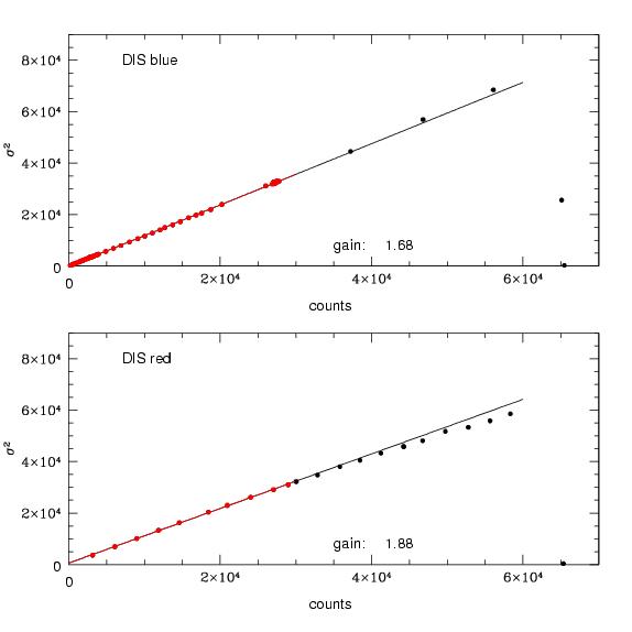
The DIS blue detector is linear up until about 50,000 DN and the DIS red detector is linear up to about 30,000 DN, as demonstrated by the following light transfer curves:
3.4. Detector Gain and Readout Noise
The light transfer test data above were obtained from a series of images taken during December 2006 and yield a gain of 1.68 electrons/DN in the blue channel and 1.88 electrons/DN in the red channel. The derived value of the gain changes slightly depending on what region of the curve is being fit. There is also always the possibility that the gain may vary slightly with time.
Pairs of bias frames yielded readout noise estimates of 4.9 and 4.6 electrons in the blue and red channels, respectively. In general, there appears to be little or no fixed (repeatable) pattern noise with the current detectors.
In the past, we have had periods where additional noise was observed to be present. If you measure significantly higher noise than is quoted here, you should notify the observing specialists and provide examples of the problem data in an effort to allow the effect to be recognized and mitigated if possible.
A measurement of the system throughput is shown for the B400/R300 grating combination in the following plot:
This plot demostrates instrument throughput before and after realuminizing the primary mirror. This should give users a feel for how much of the throughput is in the instrument and how much is in the telescope. Aside from the grating response, there is some vignetting within the cameras that leads to a reduction of throughput towards the edges of chips. As a result, the throughput for the higher resolution gratings will depend to some extent on their tilt, e.g. the chosen wavelength center. In the blue, we only have the single B1200 high resolution grating. In the red, we have both R1200 and R830; the R1200 has superior throughput at the shorter wavelength end of the red channel, while the R830 has superior throughput at the longer wavelength end, with a crossover somewhere around 7500 A.
A detailed exposure time calculator for DIS has not yet been developed. The S/N as a function of wavelength clearly depends on the spectral energy distribution of the source. In addition, seeing and choice of slit play an important role in terms of fraction of stellar light making in through the slit. For faint objects, the sky brightness, which varies with lunar phase, plays an important role. In lieu of a more detailed calculation, the signal-to-noise per pixel, in the signal-limited regime, is roughly given by:
S/N ~ 3700 10^(-0.2*m) t^(1/2) per Å in the blue channel
S/N ~ 2300 10^(-0.2*m) t^(1/2) per Å in the red channel
where these were determined for the blue spectrophotometric standard BD+28 4211. These were determined using the B400/R300 grating pair, but note that the results are quoted in S/N per Å ; thus they can be used for the other gratings to the extent that the throughput is independent of grating (as assumption whose accuracy depends on what wavelength the other gratings are used at). For S/N per pixel (after summing over the width of the spectrum), multiply the S/N above by the square root of the dispersion.
Typical DIS calibration exposures include wavelength calibration, flat fields, and bias frames. Wavelength calibration is achieved via several arc lamps that are located at the top of the telescope; in standard configuration, there are three pairs of He, Ne, and Ar lamps. In addition, two pairs of continuum quartz lamps (bright and dim) are mounted on the telescope for internal flats. Generally, the calibration lamp exposures are made with the primary mirror covers closed to yield uniform illumination. It is possible to take calibration exposures (especially wavelength calibrations) with the mirror covers open, e.g. if one wishes a reference spectrum immediately preceding or following an on-sky exposure, but the exposure levels will be fainter and the illumination less uniform. You should double or triple exposure times to compensate and also be aware that fewer arc lines will be measurable with covers open.
4.1. Calibration Lamps and Control
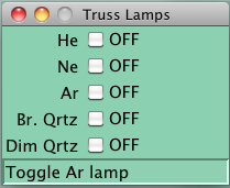
The calibration lamps are controlled by the Truss Lamps gui under Misc in the main TUI menu. In contrast with many other TUI controls, these are turned on and off by simply hitting the On/Off buttons; there is no Apply button for these lamps. The Truss Lamps gui looks like this:
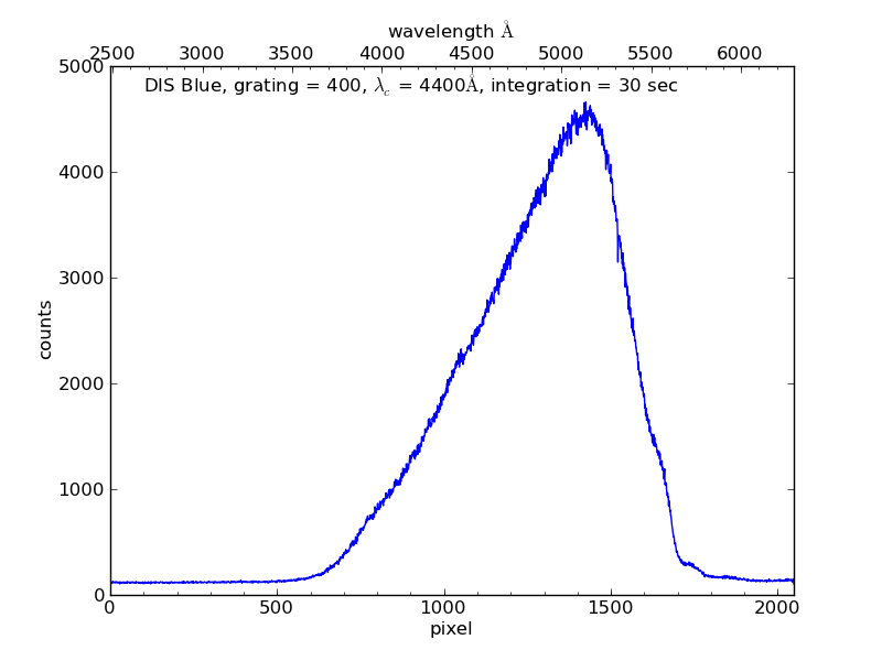
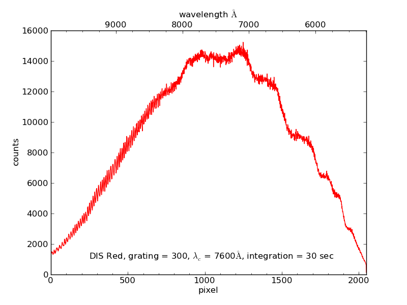
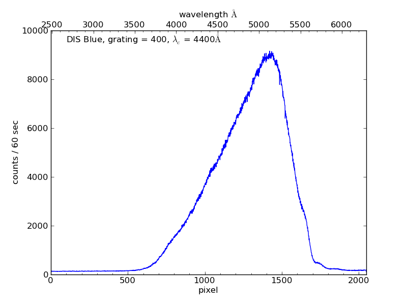
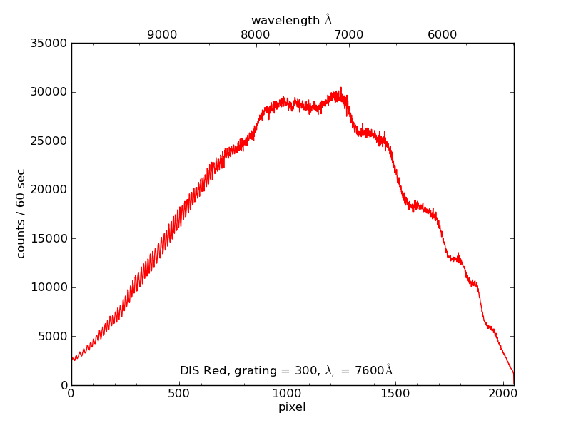
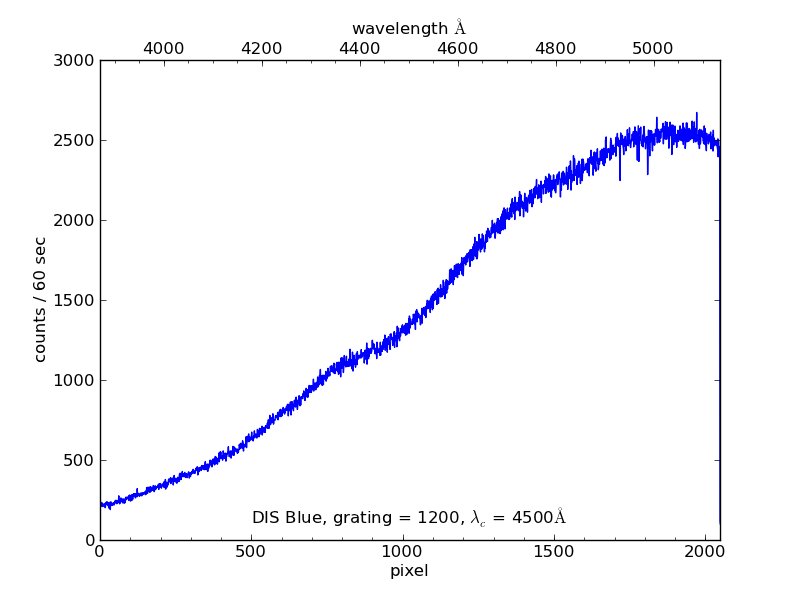
Arc lamps of He, Ne, and Ar are normally installed; we have several other lamps (H, Xe, Kr and Hg) that can be installed upon request. In the blue channel, only He provides particularly useful lines; the red channel includes lines of all 3 species. The following table includes links to typical lamp spectra for some of the standard grating setups:
Grating 30s wavecal plot 30s flatfield plot 30s wavecal plot B400 BrQrtz 4400 HgXeKrH 4400 R300 B1200 R1200
These figures in the above table show the number of counts received from each of the lamps in a 30 second exposure with the 1.5 arcsec slit.
The following table gives recommended exposure times for lamps with the 1.5 arcsec slit:
Based on this, a minimum of 60s exposure is recommended for He and Ar; Ne should not be exposed for longer than 30s if the brightest lines are in the selected spectral range. For other slits, the exposure times should be modified according to the inverse ratio of the slitsize to the 1.5 arcsec slit.
There is some small amount of internal motion within the spectrograph as the instrument is rotated on the image rotator, leading to shifts in the wavelength direction of about one pixel. Accurate wavelength calibration will require accounting for this effect. Users have the option of taking calibration lamp data at the rotator angle of each object, but in many cases, it should be possible to measure the shift using observations of night sky lines.
***The Flat Field Calibration lamps were upgraded on 2012-02-09. The tables below are updated for the new exposure times. For the previous exposure times go here.***
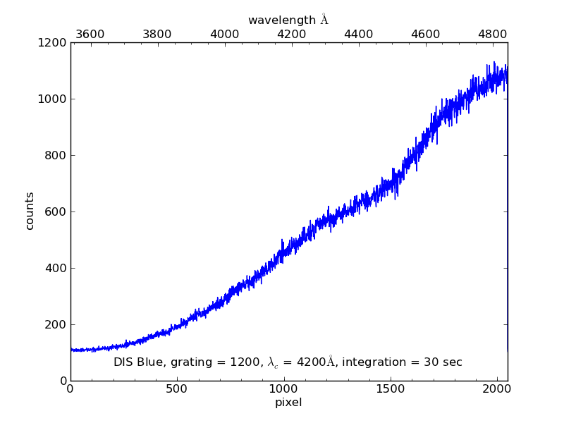
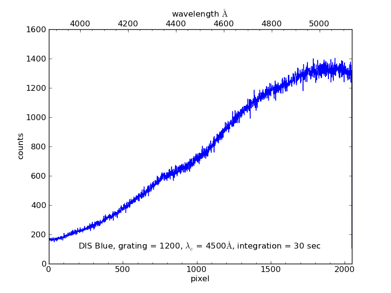
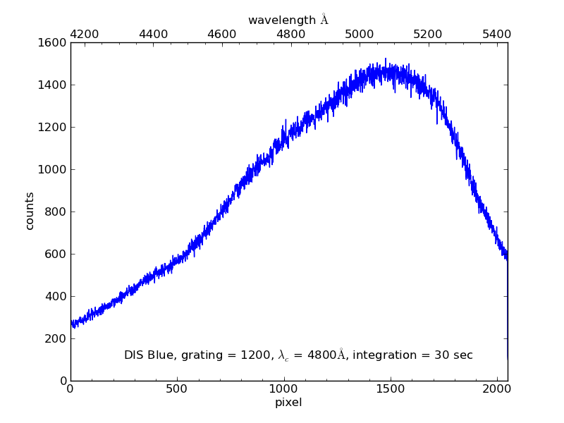
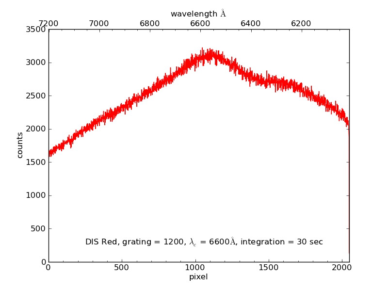
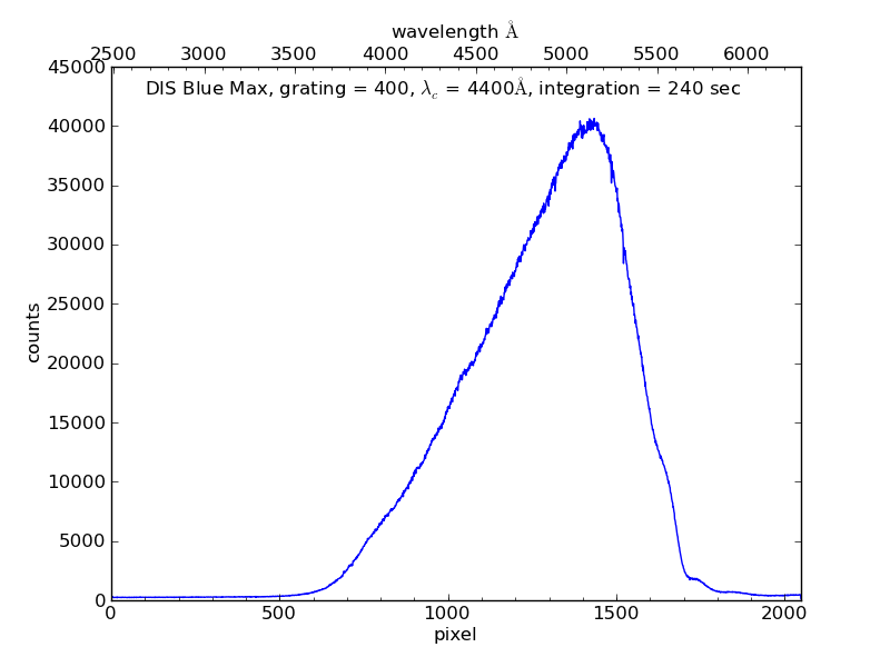
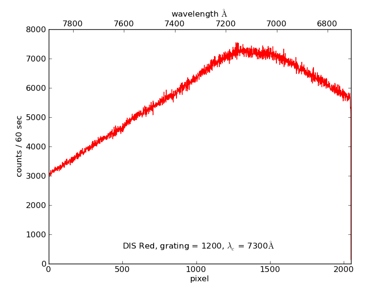
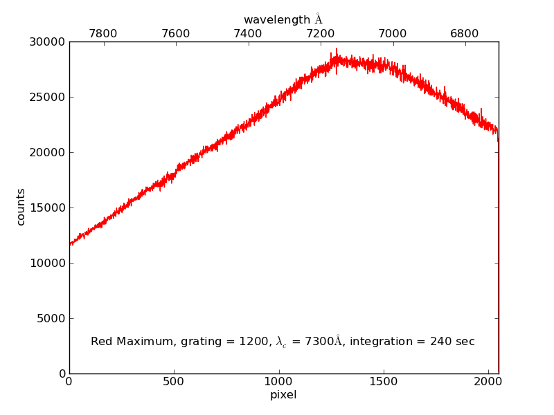
Flat fielding is generally done using the Bright Quartz lamp. The following table lists links to typical spectra for some of the standard grating setups. The lamp is moderately red, so moderately short exposures are sufficient for the red channel (e.g. 60 and 240 s for R300 and R1200, respectively). In the blue channel, there is a strong wavelength dependence; 240s will provide good flat fields longer than ~4500Å, but significantly longer exposures are needed at shorter wavelengths. (Dec 06: we are currently investigating ways to improve this situation).
| Grating | 60s flat field plot | max exp time | exp time for S/N~100 | exp time for S/N~100 | typical recommended |
|---|---|---|---|---|---|
| B400 | 190s @ 4000Å |
70s @5000Å |
5 x 100s |
||
| R300 | 20s @ 6500Å |
20s @ 8500Å |
5 x 60s |
||
| B1200 | 290s @ 4000Å |
190s @ 5000Å |
5 x 240s |
||
| R1200 | 100s @ 6500Å |
100s @ 7500Å |
5 x 240s |
||
| R830 | ? |
? @ 7500Å |
? @ 8500Å |
||
| R830 | ? |
? @ 7500Å |
? @ 8500Å |
||
The plots and exposure times are for the 1.5 arcsec slit; for other slits, the exposure times should be modified according to the inverse ratio of the slitsize to the 1.5 arcsec slit.
If you wish to do relative flux calibration for your spectra, you observe some spectrophotometric standards. Information about some standards can be found here.
A TUI catalog of the standard stars described on the above standards page.
The internal focus of the spectrograph is not adjustable by the user. Instead, spectrographs focus is a manual procedure that is done by the technical staff periodically; there are manual knobs for adjusting both the collimator and camera focus on the instrument.
Users can determine the spectrograph resolution by measuring the widths of arc lines on their wavelength calibration exposures. At best focus, the line widths should be about 2 pixels. If you find that the line widths are significantly larger than this, you should inform the APO technical staff so that they can inspect and, if necessary, adjust the spectrograph focus.
The slitviewer focus is also manually adjusted by the technical staff. There is a moderately strong variation of focus across the field of view of the slitviewer, so the focus is adjusted to bring the slit most clearly into focus. At best focus, the slit width on the slit viewer of 0.3" pixels and 1.5" slit about 5 pixels. If you observe it to be significantly wider than this, you should inform the APO technical staff.
The E2V detector installed in 2002 had very significant fringing in the red channel at wavelengths longer than about 7000Å. As a result, a new deep-depletion device was purchased from E2V and installed in December 2006. This has significantly reduced fringing (and, related, significantly higher near-IR throughput), but some level of fringing still exists at the longer wavelengths in the red channel.
It is likely that optimal strategies for removal of fringing depend on the type of exposures being obtained, e.g. if the exposures are dominated by background or by source. Some possible suggestions are to obtain flats near in time and position to your objects, and to dither your object along the slit, and subtract out sky/fringing using the dithered exposures.
5.4. Saturation in the Red Channel
When there are heavily saturated pixels in the red channel, there is significant horizontal banding seen following these pixels, even going into adjacent rows. This appears to set in at levels that would correspond to about 120,000 DN (obviously this value is not reached with the 16-bit A/D converter). As a result, observers may wish to avoid heavily saturating objects in the red.
Be sure to turn off any calibration lamps you may have used, then hand over the instrument by simply quitting out of the DIS instrument control window in TUI. In some circumstances, you may continue to use the instrument after your shift, e.g., you are the first half observer and the scheduled second-half observer is not using DIS. Ask your Observing Specialist for permission to do so if circumstances warrant.
6.1. Data Storage and Retrieval
Your data will remain on arc-gateway.apo.nmsu.edu:/export/images/your program code/UTYYMMDD/ for 9 to 12 months before being automatically deleted. Data can be accessed using scp or sftp to the institutions' observer accounts on arc-gateway (you can also use ftp and the images account and password); call APO (575-437-6822) if you are unsure of the correct login.
In general, data reduction for DIS spectra is similar to that for other long slit spectra, with some of the following basic steps:
1. Remove bias level using overscan region of chip (e.g. region (2055:2095,50:1000)).
2. Bias frames can be combined to look for fixed pattern noise, but generally this is not seen, so it may not be necessary to subtract superbias frames.
3. Wavelength calibration obtained via arc lamp observations. Note that there is significant line curvature.
4. Flat fielding can be performed using quartz lamp observations. Because of the strong spectral dependence of the quartz lamp, especially in the blue, you may wish to remove the spectral intensity dependence before flat fielding, to preserve the ability to calculate noise directly from the counts on your flat-fielded exposures.
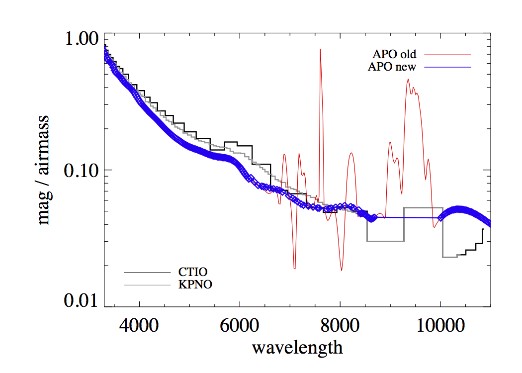
5. Flux calibration can be performed if required/desired using observations of spectrophotometric standards. You will also want to correct for atmospheric extinction at the airmass of your object. A mean extinction curve for APO has been derived for the SDSS project. The data in units of magnitude per airmass can be found here. A plot of this data, also in magnitude per airmass, can be found here. You can also plot extinction using this data. Transmission units are in fraction of flux at an airmass of 1.
6. When extracting object spectra, be aware that the spectra will likely not lie exactly along a row; there may be some tilt and/or curvature in the location of the spectrum.
7. As noted above, there is a small shift in wavelength as a function of the rotator angle (which changes across the sky even at fixed position angle). If accurate wavelength calibration is needed, consider measuring this shift using the observed position of night sky lines, or else by taking arc exposures at the position of each object.
Please find additional information for taking and reducing data here.
A. Instrument Design
Under Construction
Original instrument early 90s. Used Tek 512x512 CCD in blue, TI 800x800 CCD in red Original Documentation here.
late 90s: new gratings BM and RM purchased.
3/2002: new blue/red detectors. These are E2V 2048x1024 thinned, backside illuminated detectors.
1-5/2003: new blue/red optics, designed to better match pixel size of new detectors. Also these reduce vignetting towards the edges of the new detectors.
6-8/2006: new gratings B400, R300, R1200, purchased to better match size of new detectors and to provide improved throughput.
12/2006: new red chip, purchased to reduce fringing in the red, because the new chip is a deep depletion device. Also replace red field flattener for improved throughput. New blue prism assembly to improve UV throughput 11/06.
7/2007: new R1200 grating because previous grating was damaged.
C. Basic Low-level Commands (for scripting)
tlamps on|off 1|2|3|4|5 : Turns truss lamps on/off, Lamp1=He, 2=Ne, 3=Ar, 4=Br.Qrtz, 5=Dim Qrtz
disExpose object|flat|dark|bias t=exposure time [n=number exposures] [name=root filename]
For example, here is a simple script for taking a set of DIS calibration data:
tlamps on 1
disExpose object time=60 name=He
tlamps off 1
tlamps on 2
disExpose object time=30 name=Ne
tlamps off 2
tlamps on 3
disExpose object time=180 name=Ar
tlamps off 3
tlamps on 4
disExpose flat time=120 n=5 name=BrQrtz
tlamps off 4
disExpose bias n=10
Typical data: bias, flat, arcs, standard stars
Original DIS instrument documentation: DIS: The Double Imaging Spectrograph, Robert Lupton 1995