ARC 3.5m | GIFS
Last updated: October 2, 2014 - CAG
1. Instrument Description
The Goddard IFS and Imager (GIFS) is a visible-wavelength multi-purpose imager and imaging spectrograph for use in natural seeing at the Apache Point Observatory 3.5m telescope. As of May 2014, the instrument is available in direct imaging, coronagraphic imaging (using a wedge), and integral field spectroscopy modes. The figure shows the instrument viewed from behind together with Bruce Woodgate.
The instrument is used at the Nasmyth 2 f/10.3 focus of the APO 3.5 m telescope. Behind the telescope focus, a field lens and collimator lens collimate the light through a clear optical path, or through a lenslet array for an integral field unit. The instrument focus is wavelength-dependent, with different collimator positions to ensure collimation. A filter or other element restricting the wavelength range imaged should always be in the optical path. Finally, a camera lens refocuses the light onto the CCD, which currently can be used in a conventional analog mode. Future plans include installation of a photon-counting EMCCD camera system for photon-counting and lucky imaging.
| Mode | Spatial Sampling | Wavelength Coverage | Spectral Resolution |
| Filter Imaging | 0.165"/pixel | 4,000 - 10,000 Å | Set by filter |
| Coronagraphic Imaging | 0.165"/pixel | 4,000 - 10,000 Å | Set by filter |
GIFS uses 2 round filters, the details of which are presented in Tables 1.2-1.5. Filters noted as degraded have defects near the edge, which should be monitored for changes with time. Where known the manufacturer is specified to aid in locating filters in the storage boxes. Up to six filters can be mounted in the filter wheel at a time (Section 2.3). Please notify the observatory of your filter requests at least 24 hours in advance of your run (no later than the preceding Friday morning, if observing over a weekend). When using the IFS, the corresponding blocking filters must go in the filter slots, limiting the slots available for direct imaging.
| Filter | Wavelength (Å) | Width (Å) | Quality |
| B | 4400 | 1040 | |
| V | 5300 | 986 | |
| R | 6000 | 1545 | |
| I | 8000 | 3136 | Degraded 5mm from edge |
| Name | Measured | Manufacturer | Transmission | Quality | |
| Central Wavelength (Å) | FWHM (Å) | ||||
| filt4015 | 4020 | 50 | Andover | 48% | |
| filt4050a | 4050 | 160 | |||
| filt4050b | 4050 | 57 | Andover | 47% | |
| filt4085 | 4086 | 58 | Andover | 48% | |
| filt4120 | 4124 | 52 | Andover | 49% | |
| filt4155 | 4156 | 50 | Andover | 46% | |
| filt4160 | 4160 | 160 | |||
| filt4200 | 4206 | 108 | Andover | 55% | |
| filt4257 | 4253 | 102 | Barr | 64% | |
| filt4300 | 4313 | 116 | Andover | 60% | Degraded 8mm from edge |
| filt4400 | 4411 | 120 | Andover | 57% | Degraded 15mm from edge |
| filt4500 | 4507 | 122 | Andover | 66% | Degraded 15mm from edge |
| filt4600 | 4596 | 129 | Andover | 69% | Degraded 10mm from edge |
| filt4700 | 4701 | 109 | Andover | 76% | Degraded 10mm from edge |
| filt4760 | 4756 | 100 | Barr | ||
| filt4800 | 4816 | 107 | Andover | 77% | Degraded 10mm from edge |
| filt4865 | 4864 | 91 | Barr | 81% | Degraded 8mm from edge |
| green_ifs | 4893 | 317 | 99.06% | Green IFS blocker | |
| filt4900 | 4909 | 105 | Andover | 72% | Degraded 4mm from edge |
| filt4982 | 4982 | 15 | Degraded 5mm from edge | ||
| filt4994 | 4994 | 15 | 6mm, just one spot | ||
| filt5000 | 5007 | 106 | Andover | 74% | Degraded 4mm from edge |
| filt5007a | 5007 | 20 | Degraded 6mm from edge | ||
| filt5010 | 5011 | 106 | Barr | 74% | Degraded 3mm from edge |
| filt5020 | 5020 | 15 | Degraded 5mm from edge | ||
| filt5032 | 5032 | 15 | Degraded 8mm from edge | ||
| filt5100 | 5111 | 106 | Andover | 76% | Degraded 7mm from edge |
| filt5200 | 5210 | 116 | Andover | 72% | Degraded 10mm from edge |
| filt5265 | 5263 | 115 | Barr | 75% | Degraded 3mm from edge |
| filt5300 | 5304 | 86 | Andover | 71% | Degraded 5mm from edge |
| filt5340 | 5343 | 132 | Barr | 86% | Degraded 10mm from edge |
| filt5400 | 5406 | 124 | Andover | 74% | Degraded 5mm from edge |
| filt5500 | 5501 | 94 | Andover | 75% | Degraded 2mm from edge |
| filt5552 | 5549 | 138 | Barr | 77% | Degraded 8mm from edge |
| filt5600 | 5605 | 139 | Andover | 74% | Degraded 6mm from edge |
| filt5700 | 5703 | 139 | Andover | 74% | Degraded 2mm from edge |
| filt5800 | 5806 | 101 | Andover | 74% | Degraded 1mm from edge |
| filt5852 | 5845 | 154 | Barr | 88% | |
| filt5900 | 5902 | 109 | Andover | 76% | Degraded 1mm from edge |
| filt6000 | 6002 | Andover | 79% | Degraded 3mm from edge | |
| filt6052 | 6062 | 120 | Barr | 86% | |
| filt6056 | 6056 | 100 | Andover | Degraded 5mm from edge | |
| filt6100 | 6103 | 111 | Andover | 76% | |
| filt6200 | 6194 | 106 | Andover | 72% | ???missing from Dave's list |
| filt6245 | 6235 | 117 | Barr | 94% | |
| filt6300 | 6307 | 126 | Andover | 69% | Degraded 3mm from edge |
| filt6400 | 6403 | 116 | Andover | 68% | Degraded 2mm from edge |
| filt6455 | 6450 | 119 | Barr | 96% | |
| filt6500 | 6512 | 122 | Andover | 74% | Degraded 10mm from edge |
| halpha_a | 6564 | 10 | |||
| halpha_b | 6563 | 117 | Barr | 92% | Halpha-b |
| red_ifs | 6572 | 265 | 98 or 96%? | IFS red blocker | |
| filt6600 | 6602 | 124 | Andover | 60% | Degraded 2mm from edge |
| filt6700 | 6698 | 124 | Andover | 60% | |
| filt6702 | 6702 | 124 | Andover | 63% | |
| filt6724 | 6724 | 73 | Barr | ? | |
| filt6750 | 6750 | 200 | |||
| filt6766 | 6766 | 138 | Barr | 86% | |
| filt6800 | 6811 | 99 | Andover | 71% | Degraded 3mm from edge |
| filt6900 | 6891 | 102 | Andover | 62% | Degraded 3mm from edge |
| filt6940 | 6945 | 138 | Barr | 96% | |
| filt7000 | 7000 | 103 | Andover | 68% | |
| filt7100 | 7106 | 176 | A-wd | 95% | |
| filt7230 | 7230 | 190 | Omega | ||
| filt7240 | 7240 | 177 | ?? | 95% | |
| filt7360 | 7350 | 185 | Andover | 90% | |
| filt7480 | 7499 | 185 | Andover | 89% | Degraded 4mm from edge |
| filt7650 | 7650 | 212 | Andover | 92% | |
| filt7800 | 7785 | 218 | 98% | One side degraded | |
| filt7950 | 7964 | 235 | Andover | 96% | |
| filt8100 | 8101 | 223 | Barr | 96% | Degraded 5mm from edge |
| filt8240 | 8228 | 206 | Barr | 96% | Degraded 6mm from edge |
| filt8380 | 8368 | 244 | Barr | 92% | |
| filt8520 | 8502 | 208 | Barr | 93% | |
| filt8660 | 8668 | 218 | Barr | 94% | Degraded 8mm from edge |
| filt8840 | 8829 | 262 | Barr | 92% | |
| filt9020 | 9013 | 251 | Barr | 97% | Degraded 7mm from edge |
| filt9200 | 9200 | 316 | CS | 85% | |
| filt9380 | 9364 | 256 | Barr | 95% | |
| filt9560 | 9580 | 266 | Barr | 95% | |
| filt9770 | 9775 | 331 | Barr | 93% | |
| filt9980 | 9978 | 329 | Barr | 90% | |
| filt10190 | 10220 | 348 | Barr | 94% | |
| filt10500 | 10500 | 200 | SF | ||
| filt10830 | 10830 | 200 | A-wd | ||
| Name | Central Wavelength (Å) | FWHM (Å) | Manufacturer | Notes |
| filt4861 | 4861 | 38 | Barr | Hβ |
| filt5007b | 5007 | 40 | OIII | |
| halpha_c | 6563 | 63 | Barr | at GSFC |
| filt6724 | 6724 | 73 | Barr |
| Name | Central Wavelength (Å) | FWHM (Å) |
| York5059 | 5060 | 12 |
| 430-610nm/Interference | 5200 | 1800 |
| York5202 | 5202 | 13 |
| York5685 | 5685 | 14 |
| York5720 | 5720 | 14 |
| CU5893 | 5893 | 15 |
| York5917 | 5915 | 20 |
| York6007 | 6008 | 15 |
| York6178 | 6008 | 15 |
| York6409 | 6008 | 15 |
| York6569 | 6569 | 15 |
| CU6731 | 6731 | 15 |
| York6903 | 6903 | 17 |
| York6931 | 6929 | 17 |
| 600-940nm/Interference | 7700 | 3400 |
| York7740 | 7740 | 19 |
| York8212 | 8207 | 20 |
| York8238 | 8236 | 20 |
| York8678 | 8662 | 21 |
| York9088 | 9089 | 22 |
Observers wishing to use their own filters (2 diameter, round) should contact Bill Ketzeback at APO.
GIFS can also be configured as an IFS with choice of 14 x 14 or 7 x 7 fields of view. The IFS operates in the green and red (λ ≤ 7000 Å). A slot partially illuminating the lenslet array can be manually installed in the instrument to enable broader wavelength coverage over a reduced field of view.
| FOV (arcsec x arcsec) | Spatial Resolution (arcsec/spaxel) | Spectral Bandwidth (Å) | Spectral Sampling (Å) | Central Wavelength (Å) | Spectral Coveragea (Å) | Modeb | Lines in Range |
| BLUE/GREEN grating R~1475 | |||||||
| 7" x 7" | 0.215 | 310 | 1.05 | 4890 | 4740-5040 | NSG | Hβ, [O III] |
| 14" x 14" | 0.43 | 310 | 1.05 | 4890 | 4780-5040 | WSG | Hβ, [O III] |
| 7" x 1.68"c | 0.215 | 107 | 1.05 | 4890 | 4330-5400 | NLG | Hβ, [O III], Fe XIV, Ar IV, He I, Cl III, Fe III, He II, Ne IV |
| 14" x 3.36" | 0.43 | 107 | 1.05 | 4890 | 4330-5400 | WLG | Hβ, [O III], Fe XIV, Ar IV, He I, Cl III, Fe III, He II, Ne IV |
| RED grating R~1823 | |||||||
| 7" x 7" | 0.215 | 420 | 1.44 | 6640 | 6430-6850 | NSR | Hα, [N II], [S II] |
| 14" x 14" | 0.43 | 420 | 1.44 | 6640 | 6430-6850 | WSR | Hα, [N II], [S II] |
| 7" x 1.68"c | 0.215 | 1250 | 1.44 | 6640 | 5750-7000 | NLR | +[O I], [S III], FeX, He I |
| 14" x 3.36" | 0.43 | 1250 | 1.44 | 6640 | 5750-7000 | WLR | +[O I], [S III], FeX, He I |
The bare lenslet array has higher throughput than the pinhole array, but has some light scattered and diffracted into the inter-spaxel region. Each spaxel illuminates more than one pixel, but spaxels illuminate fewer pixels with the pinhole array in place than with the bare array in place. The ratio of pinhole/bare throughput is 77% at the peak pixel, but when light from a given spaxel is integrated over all the pixels, the throughput ratio is 72%. This loss in transmission is due to the mask blocking scattered light outside the core. The bare lenslet array also has a smudge in the lower left quadrant, and the team is working to correct it. In the meantime, observers are advised to keep targets out of the affected area as necessary.
1.3 Comparison with Other APO Facility Instruments
As an imager, GIFS has a circular field of view which is only ~60% that of SPICAM. The main strength of GIFS as an imager in analog mode is the large suite of medium-band filters (FWHM=135Å) and the availability of the coronagraphic wedge, or in the future as an imager with photon-counting and lucky imaging modes. As an IFS, GIFS offers contiguous 2-D spatial coverage of a field which is larger than the DIS slit widths, with higher spectral resolution than DIS, but with wavelength coverage limited to the green and red. DIS offers more complete (or user-specified) wavelength coverage, and simpler target acquisition and data analysis, at the expense of less complete spatial sampling near an object of interest.
| Instrument | Field of View | Filter Complement | Spectral Resolution |
| SPICAM | 4.7' | SDSS u'g'r'i'z' MSSSO UBVRI | Few; set by bandpass |
| GIFS Imaging | 1.7' x 1.7' with some vignetting | BVRI, medium band | ~2-3 for broadband ~20 grating blockers 48 medium band, red 70 Rutgers broad blockers and higher for a few filters |
| DIS | 1.5", 2", or 5" x 6' | Long-slit | 300-400, 1200 0.4 - 1.0 microns simultaneously |
| GIFS as IFS | 14" x 14" or 7" x 7" | IFS | R = 1475 (green) R = 1823 (red) R = 5000 (hi-res) |
Software Control for GIFS is provided by the Telescope Users Interface (TUI) package written by Russell Owen (UW). Commanding for GIFS requires version 2.3.1 or later. You can check which version you are running by pulling down TUI>>About TUI on the main menu bar.
At startup, TUI produces a selection of windows to control the telescope, the science instrument, and the calibration lamps, to provide messaging with the observing specialist, and command line commanding of the science instrument.
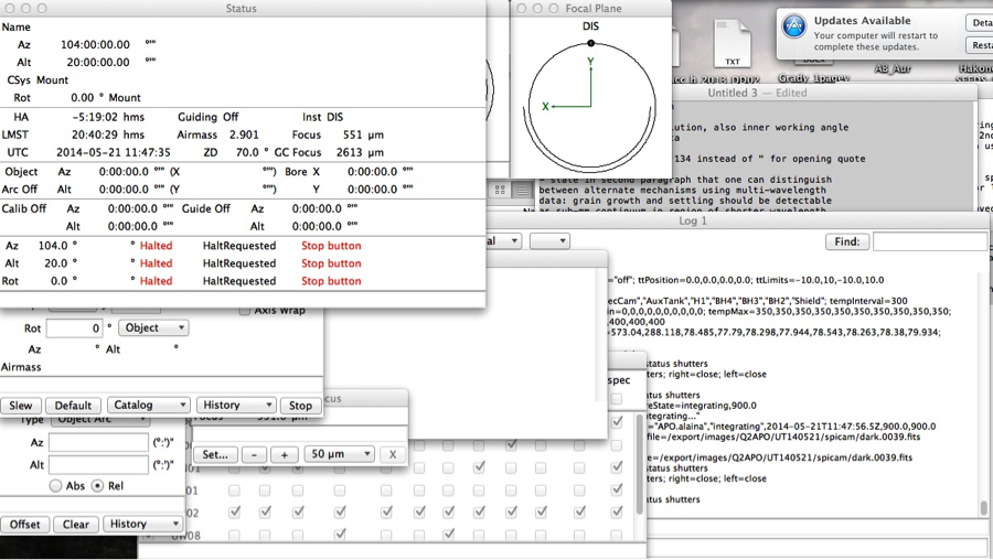 |  |
| TUI at startup | Telescope pointing and status information is located on the Status window. |
Using the "Inst" pull down menu on the menu bar, select GIFS (Inst>>GIFS). This brings up the GIFS configuration window. You should see a display similar to Figure 2.2.1a with a list of mechanisms on the left and values on the right.
 | 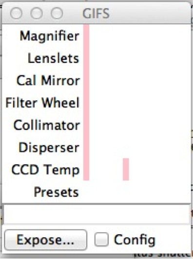 |
| Current instrument status should be shown. | If this is what you see upon launching GIFS, the GIFS actor needs to be restarted; ask the observing specialist |
If no data are shown (Figure 2.2.1b), and where they should appear is pink, you will need ask the observing specialist to restart the GIFS actor.
Magnifier, lenslet, and disperser values are normally changed using preset instrument configurations, which can be accessed using the "Presets" pull-down menu, while the filter in the optical path can be changed using the "Filter Wheel" pull-down menu.
Changes to configurations are first selected, at which point they will have a colored background. Actually moving the mechanism is done using the "Apply" button at the bottom of the GIFS window. At this point, you will see count down timers appear and count down as the mechanisms individually move.
The GIFS initial default is that the "Config" box is not checked. To change the instrument configuration, tick the "Config" box.
The six filters you requested to be mounted are listed in the "Filter Wheel" pull-down menu and are named as specified in the confirmation email from the observatory. Click on the filter you want, and then press "Apply." Wait until the countdown timers have counted down and there is no colored background to the filter pull-down menu before changing other configurations. Filter changes normally result in automatic changes to the collimator setting to compensate for the change in instrument focus.
Configuring GIFS for either filter imaging or IFS spectral imaging requires coordinated movement of several of the mechanism drives. Present configurations for the most heavily used of these modes have been defined and can be accessed via the "Presets" pull-down menu on the GIFS window. These include options for direct imaging with and without a coronagraphic wedge in the optical path, Fabry-Perot operation (not currently available), and use of the IFS with its choice of 2 magnifications (14/7), 2 lenslet arrays (bare/pinhole), and imaging or spectroscopic modes. The syntax of the presets is generally:
mode,magnification,lenslet,disperser,collimator
Table 2.1: Preset Instrument Modes Preset Command Mode Use Direct_imaging,clear,collg Direct imaging Initial target acquisition in green Direct_imaging,clear,collr Direct imaging Initial target acquisition in red Direct_imaging,wedge,collg Direct coronagraphic imaging Coronagraphic imaging in green Direct_imaging,wedge,collr Direct coronapgraphic imaging Coronagraphic imaging in red fp,wedge,collg Fabry-Perot imaging Not available at this time fp,wedge,collr Fabry-Perot imaging Not available at this time fp,wedge,collg Fabry-Perot coronagraphic imaging Not available at this time fp,wedge,collr Fabry-Perot coronagraphic imaging Not available at this time ifs,14,bare,clear,collg
ifs,7,bare,clear,collgIFS acquisition (no disperser, no pinhole mask) Source placement in field of view in green ifs,14,pinhole,clear,collg
ifs,7,pinhole,clear,collgIFS acquisition (no disperser, with pinhole mask) Source placement in field of view in green ifs,14,bare,clear,collr
ifs,7,bare,clear,collrIFS acquisition (no disperser, no pinhole mask) Source placement in field of view in red ifs,14,pinhole,clear,collr
ifs,7,pinhole,clear,collrIFS acquisition (no disperser, with pinhole mask) Source placement in field of view in red ifs,14,bare,green
ifs,7,bare,greenIFS spectrum (disper in place, no pinhole mask) Spectral imaging in green ifs,14,pinhole,green
ifs,7,pinhole,greenIFS spectrum (disper and pinhole mask in place) Spectral imaging in green ifs,14,bare,red
ifs,7,bare,greenIFS spectrum (disperser in place, no pinhole mask) Spectral imaging in red ifs,14,pinhole,red
ifs,7,pinhole,redIFS spectrum (disperser and pinhole mask in place) Spectral imaging in red GIFS exposures can be specified by clicking on the Expose button at the bottom of the GIFS window. The process is similar to other instruments at the ARC 3.5m telescope. This launches the GIFSExpose window. You can specify the image type (object, flat, dark, or bias), the integration time, the number of exposures, the name and a comment to be added to the FITS header. Files with names of the form "name.####.fits," where "####" is a running number, will be created at the end of the integration in a directory named with the current UT date. Files are temporarily archived at APO and are downloaded to a path on your machine which can be selected under TUI>>Downloads>>.
GIFS supports direct filter imaging using the filter list in Section 1.1, with up to six filters mounted at a time. If you plan to combine direct imaging with IFS use, you will need to allocate a filter slot for blocking filters for each IFS grating that you will be using. Direct images can be made in either direct imaging mode or coronagraphic imaging mode.
In general, the process is:
- Slew to your target and request guiding.
- Select filter and configure instrument for imaging using one of the "direct_imaging" presets.
- Initial acquisition of target.
- Offset to place target at preferred location in field of view (as needed).
- Expose as required.
The IFS component consists of two sections, the pre-formatter optics and the spectrograph. The pre-formatter section magnifies the image from the telescope focus onto a microlens array, so that the lenslets act as spatial samples in an image plane. This design follows the TIGER design concept (Bacon, R., et al. 1988, The Integral Field Spectrograph TIGER, in ESO conference VLTs and their instrumentation, Munich, March 1988.), similar to OSIRIS at Keck (Larkin, J.E., et al. 2003, OSIRIS: Infrared integral field spectrograph for the Keck adaptive optics system SPIE, 4841, 1600.54), where spectra are interleaved between concentrated image points.
The spectrograph uses existing GIFS optics such as the field lens, collimator lens, band-limiting filters in the existing filter wheel, and a camera to focus the images onto a back-illuminated EMCCD. The spectrograph portion of the IFS is located on the disperser drive behind the filter wheel in the parallel beam section of the instrument, and consists of three IFS dispersers, one for the red_ifs, one for the green_ifs and one for a higher resolution red ifs (hires), as well as supporting a clear path for direct imaging. Each IFS disperser consists of a transmissive grating, between two prisms to return the dispersed light to its original path in both rotation and translation. The gratings use Volume Phase Holograph technology for transmission and high throughput.
The lenslet arrays concentrate light into image spots that act as the input to the spectrograph. The grid of image spots can be observed without dispersion, as in the target acquisition sequence for the IFS, or dispersed such that the spectra are spatially separated on the detector. At most, we can have 32x32 spatial samples, 1024 spectra, on the detector in a single frame. The lenslets are on a regular grid, and sample the image plane like a detector. In analogy with detector pixels, the lenslet images are termed spaxels (i.e., spatial elements) in the rest of this document.
The observer may choose between two magnification modes: 14"x14" or 7"x7". For most purposes, the larger magnification is better, due to the typical APO seeing limit and accuracy of offset maneuvers. On a night with particularly good seeing or on targets that are bright, and not read-noise-limited, the 7"x7" may be preferable.
Integral field spectroscopy with GIFS is more complex than direct imaging. In general, the data acquisition process is:
- Slew to your target and request guiding.
- Select filter and configure instrument for imaging using the blocking filter that you will be using with the IFS grating.
- Take initial direct image.
- Use the "Offset" window to offset pointing to put the target at (x,y)=(420,496) in the direct imaging field of view. Confirm you moved to the correct location on the detector with another direct image (and the help of an observing specialist).
- Configure GIFS for IFS acquisition with your preferred magnification (14" or 7"), choice of lenslet array (bare or pinhole), and green or red collimator.
- Take an IFS acquisition image ("clear," no disperser in place) to locate your target in the field of view. The IFS field of view is rotated with respect to the direct imaging field by 187 degrees. Exposure durations can be ~2-4x shorter than your initial acquisition image, due to image compression by the spaxels. The orientation of the IFS on the sky is rotated with respect to the direct imaging configuration by 187°, due to a combination of the optics and the orientation of the lenslet array. If you wish, examine the image using the GIFS DRP
- Configure the instrument for spectral imaging.
- Take spectral images.
- Turn on truss lamp for wavelength calibration and spectral trace data.
- Take wavelength calibration and spectra trace data.
- Repeat science target observations as needed.
- Reduce IFS spectral data using the GIFS DRP.
The telescope is focused by inspection of images taken in direct imaging mode. Generally, focusing is most efficiently accomplished by asking the Observing Specialist to focus the telescope. The observing specialist can run the GIFS focus script to expedite the process and provide a current seeing estimate.
As with all instruments, monitoring focus is advisable. The telescope focus will change over the course of the night, especially at the beginning of the night when the telescope is changing temperature.
GIFS guiding is performed using the NA2 guide camera. You will need to request guiding.
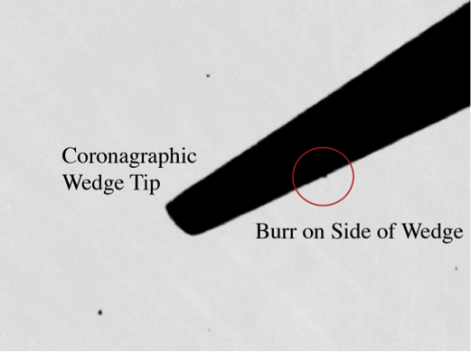
The GIFS coronagraphic wedge has a small burr on its underside (x,y)=(498,541), (Figure 3.2.1) which we use for collimator focus checks for wavelengths < 9,000 Å
The instrument's focus is wavelength dependent. As a result, the collimator must be adjusted to achieve proper focus for any given filter/lenslet/grating combination. The ICC/TUI will set the focus automatically. If a filter is loaded, and the direct image seems blurry (e.g. can't see the burr), contact Bill Ketzeback at APO. This is particularly important if you are using the filters in table 1.5, or your own filters.
3 Instrument PerformanceSlews to targets are controlled using the TUI Slew window (Figure 2.10.1), either by manually specifying target coordinates or by providing an ASCII file with target coordinates, which can be selected using the "Catalog" button at the bottom of the window. The default field rotation places E-W in the detector x-direction. This can be altered by specifying a rotation angle in the TUI Slew window.
Figure 2.10.1: Navigating to Targets in TUI TUI Slew Window TUI Offset Window It is necessary to offset from the acquired coordinate location of the target to the IFS aperture sweet spot at (x,y)=(420,496). Use the TUI Offset window (Figure 2.10.2) to input either an "Obj Arc" or "Boresight" offset in pixel or angle increments. For conversion from pixel location to offsets in arcseconds, the pixel scale is 0.165 in direct imaging mode. The location of the IFS aperture is not immediately apparent in GIFS direct images, but is just off the tip of the coronagraphic wedge, allowing for another method of properly placing your target on the IFS when the wedge is in place. No matter the absolute coordinate of the sweet spot, the relative offset between the coronagraphic burr and the sweet spot remains constant. From the burr, the sweet spot should be at (δx,δy)=(-78,-45) in pixel coordinates.
3.1 Detector Summary with Leach (analog) electronics
Table 3.1: Detector summary with Leach (analog) electronics Detector e2v CCD201 Serial Number Number of rows 1024 Number of columns 1024 Pixel Size 13.3μm x 13.3μm Gain 2.3e-/ADU Readout noise 2.88e- Dark Current 1e-/pixel/hour Linearity Regime < 30,000 DN Full Well (=34.78Ke/gain) 80,000 e- Chip QE
4000 Å
5000 Å
6500 Å
9000 Å
52%
90%
91%
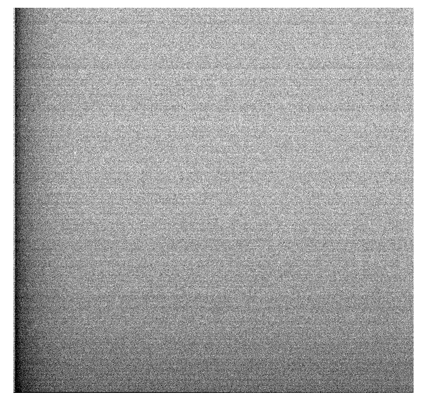
35%Readout time 18 seconds Default Analog Mode Timing File fwd5_0.lod The optical center of GIFS and the CCD center are not perfectly aligned. There is vignetting of the image, reaching up to 57% light loss compared to the center of the field: this can be compensated with flat field images obtained using the BrQtz lamp. There are no known bad columns or hot pixels as of May 2014. However, there are some dust specks visible. Fringing is seen with very narrow band or very red filters.
Figure 3.2.1: GIFS Detector Response x y 544 555 462 376 176 218 636 265 531 868 731 343 941 137 Flat field response of detector with and without coronagraphic wedge in place. Note the presence of vignetting. Close-up of coronagraphic wedge and the burr on the side. The burr is a fortuitous defect helpful in focusing Dust speckle locations (pixel coordinates).
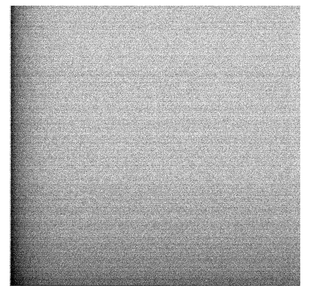
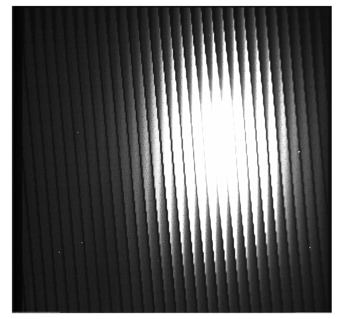
Figure 3.2.3: GIFS Detector Bias Frames Example bias frames. Note the striping (and its variation from frame to frame). A bias removal IDL-based script which uses the reference pixels is provided in the data distribution. See the GIFS DRP for more details.
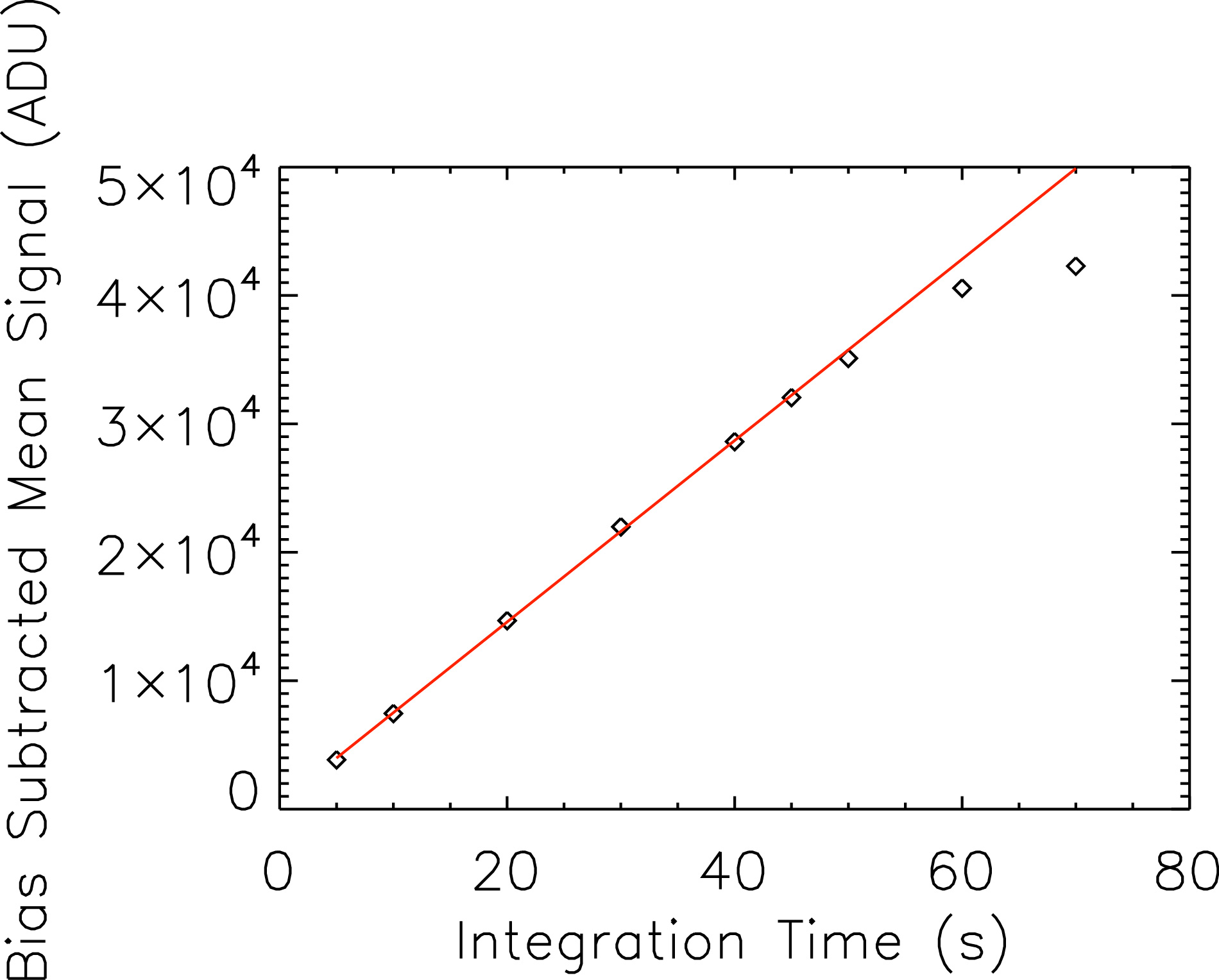
Figure 3.2.2: GIFS Detector Linearity Detector response plotted against bright quartz truss lamp integration time, As measured for a 51x51 pixel box centered on (x,y)=(425,475). To ensure linearity, exposures should be kept under 34k ADU. Standard deviations for each point plotted are smaller than the plot symbol used. To avoid saturation after lamp replacement in Feb. 2012, integration times should be 75% of the values shown above. 4 Instrument Calibration
Table 3.3: Representative Integration Times: Direct Imaging Source Type Integration Time (s) Exposure Level (photometric conditions) BD+28 4211
R=10.6, V=10.5
Red Grating Blocker5 Peak single pixel: 15k DN over bias
Integrated over point source: 1.12e7 DNDG Tau, T Tauri star
R=11.4
Hα30 Peak single pixel: 22.2k DN over bias
Integrated over point source: 9.38e5 DNStandard Star (HZ 44)
V=11.47
Green Grating Blocker5 Peak single pixel: 6500 DN over bias
Integrated over point source: 366k DN4.1 Calibration Lamps and Controls
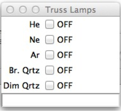
GIFS uses the truss lamps on the 3.5m for wavelength, flat field, and spectral trace observations. Truss lamp controls are found under Misc>>Truss Lamps on the TUI menu bar (Figure 4.1.1). Individual lamps can be turned on and off independently.
Figure 4.1.1: TUI Truss Lamp Window 4.2 Direct Imaging Calibration
Observers will need bias frames, flat field frames, and observations of standard stars. Bias frames show a 10 ADU gradient top to bottom, and a 4DN gradient along rows, as well as low-level striping. Bias frames are actually 100ms darks, and can contain isolated cosmic ray events. We suggest using a median of an odd number of bias frames as a super bias, and then explore destriping algorithms. Raw analog images have 1072x1032 pixels, including 16 pixels of overscan plus 16 pixels of dark reference (i.e., aluminum covered pixels). On the right hand side of the image are another 16 pixels of overscan. The top of the image has another 8 row-wide dark reference strip. These strips can be used as alternates to dedicated bias frames or dark frames, but will not fully account for the striping. The active image area corresponds to pixels x=33-1056, y=0-1023.
Flat fields are typically obtained using the Bright Quartz truss lamp. Integration times depend on choice of blocking filter, but nominal values are given in Table 4.2.
Table 4.2: Representative Integration Times: Imaging Calibrations Red Blocking Filters Green Blocking Filters Flat Field -- Bright Quartz Lamp 2s gives 10,000 counts over bias 9s gives 10,000 counts over bias To reduce IFS data, observers need to take the same calibration data as when performing direct imaging (bias, flat field, and standard star frames). Additionally, you must take IFS acquisition images with the bright quartz lamp to locate the spaxels, wavelength calibration data (He, Ne, and Ar lamps on, disperser in place) with each grating/filter used, and trace observations (at least 200 counts over bias, bright quartz lamp on and dispersing grating in place) with each grating used. Analog IFS observations use a combination of emission line spectra for wavelength calibration and bright quartz observations to locate individual spectra (trace).
Table 4.3: Representative Integration Times: IFS Calibrations Red grating Green grating Spectral Trace -- Bright Quartz Lamp 7.5s gives 200 counts over background 112s gives 200 counts over background Wavelength Calibration Ne 30s gives 2k counts over background
S/N=100 in 150sHeNe 150s gives 450 counts over bias for brightest line
S/N=30 in 300sIf you wish to perform relative flux calibration for your spectra, you must observe some spectrophotometric standards. Information about standard stars can be found here.
A TUI catalog of standard stars is described on the above standards page.
5 Instrument Issues
Table 4.4: Nominal Integration Times for V=10.5 Continuum Source, Bare Lenslet Array, and 14" x 14" FOV IFS Acquisition 10s to S/N=100 per spaxel Red grating 900s to S/N=100 per dispersed pixel Green grating 600s to S/N=100 per dispersed pixel 6 End of Your RunNo known hot pixels or bad channels as of August 2014.
Be sure to turn off any calibration lamps you may have used, and then hand over the instrument by simply quitting out of the GIFS instrument control window in TUI. In some circumstances, you may continue to use the instrument after your shift. For example, if you are the first half observer and the scheduled second-half observer is not using GIFS. Ask your observatory specialist for permission to do so if circumstances warrant.
Data reduction for IFS observations is complex. We have developed an IDL-based software package to handle the conversion of the observations into data cubes, and a manual for its use. Click here to go to the GIFS Data Reduction Pipeline (DRP) Manual The IDL-based package can be requested by emailing the GIFS Team. It will be available at this site for direct download soon.Your data will remain on newton.apo.nmsu.edu:/export/images/your program code/UTYYMMDD/ for 9 to 12 months before being automatically deleted. Data can be accessed using scp or sftp to the institutions' observer accounts on newton (you can also use ftp and the images account and password); call APO (575-437-6822) if you are unsure of the correct login.
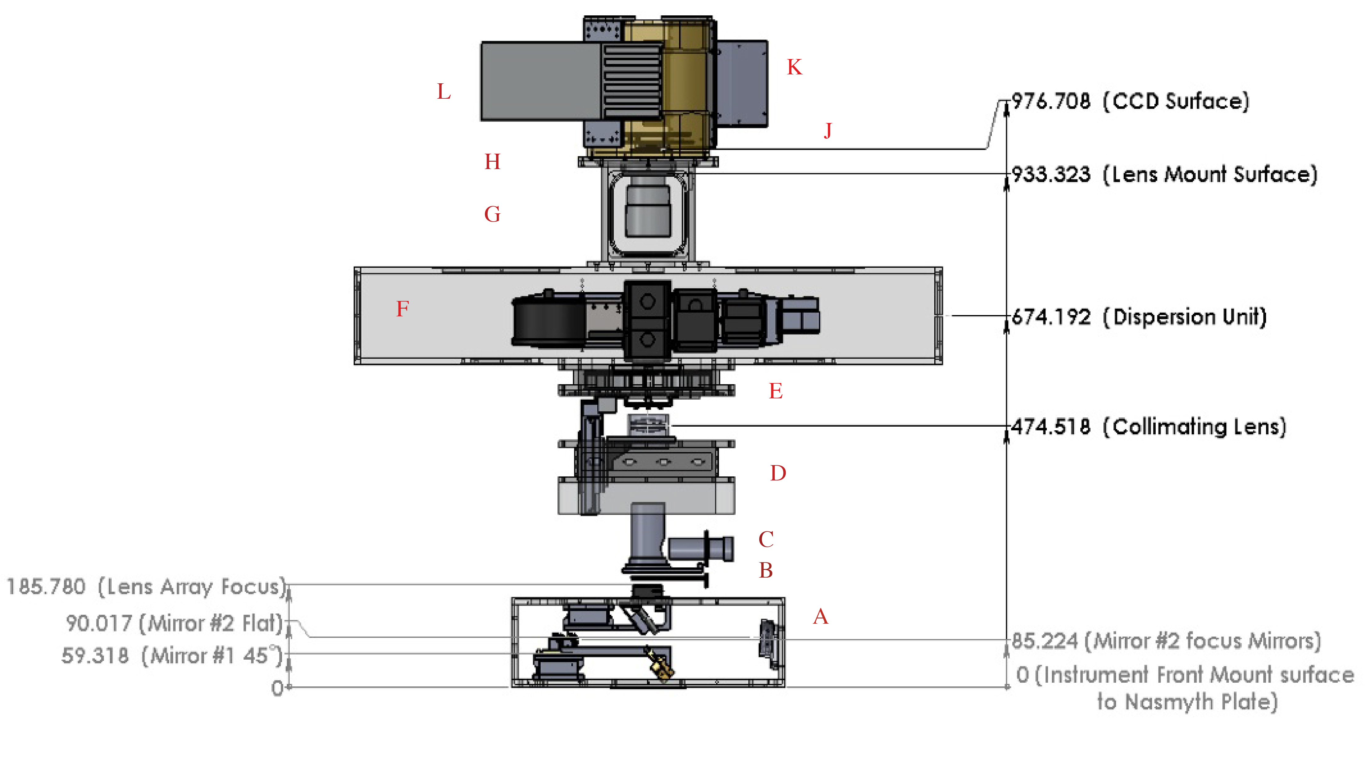
Figure A.1: Instrument Schematic SolidWorks view of GIFS from bottom (telescope) to detector (top): Box A (magnifier drive) houses IFS lenslets and associated optics, a coronagraphic wedge for direct imaging and a clear path for conventional filter imaging. B is the manual slider for alternate coronagraphic spots. C is the location of the internal calibration system that is not currently being utilized. Box D houses the collimating lens and its associated focus drive. E is the filter wheel. F is the disperser drive housing IFS VPH gratings, and a clear path for conventional imaging. G is the camera lens. H is the shutter assembly and camera lens mount. J is the CCD in its dewar. K is the Photon ETC controller for the CCD (not currently used), and L is the Leach controller (currently used). The instrument image planes are at the lenslet array (See Box A) for all modes and at the CCD surface. The filter wheel is located near the pupil plane.
Figure A.2: Optical Layout (IFS Mode) Simplified optical diagram for the low-resolution red IFS mode. In TUI, two scripts are available to GIFS users, both found by navigating on the menu bar to Scripts/GIFS/. Both are nodding scripts, utilizing an ABBA nod pattern. One ("Nod_Objarc") uses an "objarc" offshift, while the other ("Nod_boresight") uses a boresight offshift. Users may implement their own personal Python scripts by navigating to Scripts/Open.
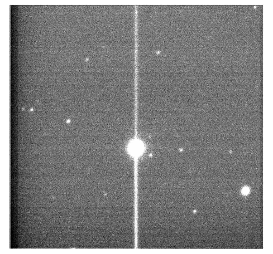
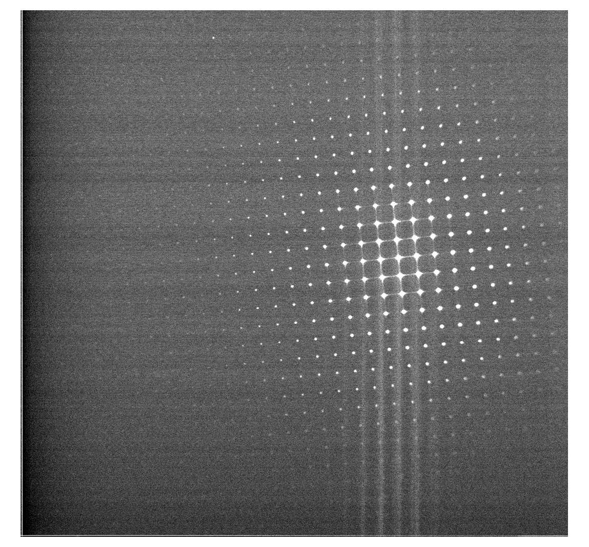
Figure C.1: GIFS Data Examples Direct Imaging IFS Acquisition Mode ("clear") IFS Spectral Mode ("bare") The present GIFS instrument is the reincarnation of the Goddard Fabry Perot (GFP). The NASA APRA program supported the GIFS upgrade, which matures integral field spectroscopy and photon counting detector technologies. The team working on this instrument has been co-located at NASA Goddard and was led by Bruce Woodgate. The team now includes Michael McElwain (PI), Carol Grady, James Bubeck, Don Lindler, Jorge Llop, Michael Malatesta, George Hilton, Tim Norton, Ashlee Wilkins, and John Wisniewski.Sample FITS Header:
SIMPLE = T / file does conform to FITS standard BITPIX = 16 / number of bits per data pixel NAXIS = 2 / number of data axes NAXIS1 = 1072 / length of data axis 1 NAXIS2 = 1032 / length of data axis 2 EXTEND = T / FITS dataset may contain extensions OBSERVAT = 'APO' / Per the IRAF observatory list. TELESCOP = '3.5m' INSTRUME = 'gifs' / Instrument name LATITUDE = +3.2780361000000E+01 / Latitude of telescope base LONGITUD = -1.0582041700000E+02 / Longitude of telescope base TIMESYS = 'TAI' / Time system for DATE-OBS UTC-TAI = -35.0 / UTC = TAI + UTC_TAI(seconds) UT1-TAI = -35.28 / UT1 = TAI + UT1_TAI(seconds) LST = '12:58:07.518' / Local Apperent Sidereal time OBJNAME = 'HD189733' / Object name, per TCC ObjName RADECSYS = 'FK5' / Coordinate system, per TCC ObjSys EQUINOX = +2.0000000000000E+03 / Equinox, per TCC ObjSys OBJANGLE = +1.0460000000000E-03 / Angle from inst x,y to sky RA = '20:00:43.68' / RA hours, from TCC ObjNetPos DEC = '22:42:35.44' / Dec degrees, from TCC ObjNetPos ARCOFFX = +2.5000000000000E-03 / TCC arc offset X ARCOFFY = +5.6100000000000E-04 / TCC arc offset Y OBJOFFX = +0.0000000000000E+00 / TCC object offset X OBJOFFY = +0.0000000000000E+00 / TCC object offset Y CALOFFX = +0.0000000000000E+00 / TCC calibration offset X CALOFFY = +0.0000000000000E+00 / TCC calibration offset Y BOREOFFX = +0.0000000000000E+00 / TCC boresight offset X BOREOFFY = +0.0000000000000E+00 / TCC boresight offset Y AIRPRESS = +7.3156000000000E+04 / Air pressure, Pascals HUMIDITY = +3.9000000000000E-01 / Humidity, fraction TELAZ = -2.5168000000000E+01 / TCC AxePos azimuth TELALT = +7.9071000000000E+01 / TCC AxePos altitude TELROT = +5.6264000000000E+01 / TCC AxePos rotator TELFOCUS = +5.2500000000000E+02 / TCC SecFocus ZD = +1.0929000000000E+01 / Zenith distance AIRMASS = +1.0184721546228E+00 / 1/cos(ZD) CTYPE1 = 'RA---TAN' / WCS projection CTYPE2 = 'DEC--TAN' / WCS projection CRPIX1 = +5.5090000000000E+02 / WCS reference pixel CRPIX2 = +4.1490000000000E+02 / WCS reference pixel CRVAL1 = +3.0018471800000E+02 / WCS reference sky pos. CRVAL2 = +2.2710405000000E+01 / WCS reference sky pos. CD1_1 = -4.4585731666720E-05 / WCS (1/InstScaleX)*cos(InstAng) CD1_2 = +8.3068183875392E-10 / WCS (1/InstScaleY)*sin(InstAng) CD2_1 = +8.1396353666715E-10 / WCS (-1/(InstScaleX)*sin(InstAng) CD2_2 = +4.5501494716519E-05 / WCS (1/InstScaleY)*cos(InstAng) COMMENT FITS (Flexible Image Transport System) format is defined in 'Astronomy COMMENT and Astrophysics', volume 376, page 359; bibcode: 2001A&A...376..359H BZERO = 32768 / offset data range to that of unsigned short BSCALE = 1 / default scaling factor SECTION1 = '///////////////// GFP/IFS astrometry information //////////////' FIMPIX = '0.165 arcsec/pix' / Filter imaging pixel scale IFS14SS = '0.0139 arcsec/pix' / IFS 14x14 spaxel scale IFS7SS = '0.00688 arcsec/pix' / IFS 7x7 spaxel scale IFS14LS = '0.43 arcsec/lenslet' / IFS 14x14 lenslet scale IFS7LS = '0.215 arcsec/lenslet' / IFS 7x7 lenslet scale FIMSSX1 = '570 ' / Filter_imaging_sweet_spot X1 FIMSSY2 = '480 ' / Filter imaging sweet spot Y1 IFSDR = '172.87 or 187.12 degrees' / IFS_Delta_Rotation SECTION2 = '//////////////// Science instrument configuration /////////////' INST = 'gfp-ifs ' / Goddard Fabry-Perot-Integral Field Spectrograph M_POS = 8003 / Numerical position of Magnifier M_TYPE = '14x14 ' / Magnifier preset name L_POS = 168980 / Numerical position of Lenslets L_TYPE = 'bare_lens' / Lenslets preset name D_POS = 727420 / Numerical position of Disperser D_TYPE = 'green ' / Disperser preset name OBS_MODE = 'IFS ' / Observation Mode - IFS, IFS_ACQ, F-P or CLEAR F_POS = 1 / Position of filter on wheel FILTER = 'GREEN_IFS' / Filter element type FWAVE = '4893 ' / Filter center wavelength F_FWHM = '317 ' / Filter full-width at half max CALMIRR = 'OUT ' / Setting of calibration mirror SECTION3 = '////////////// Fabry-Perot parameters ////////////////' ETALON = ' ' / Fabry-Perot etalon ETALPOS = ' ' / Etalon position FPX = ' ' / Fabry-Perot X setting FPY = ' ' / Fabry-Perot Y setting FPZ = ' ' / Fabry-Perot Z setting FPTEMP = ' ' / Fabry-Perot etalon temperature AIRTEMP = ' ' / Fabry-Perot air temperature FPCALZER = ' ' / Fabry-Perot calib zero point offset FPCALN = ' ' / Fabry-Perot Y setting FPW = ' ' / Fabry-Perot Z setting GFPX0 = 0.0 / X optical center GFPY0 = 315.0 / Y optical center GFPF = ' ' / Gradient LAMP = ' ' / Calibration lamp XCOARSE = ' ' / CS-100 X course XFINE = ' ' / CS-100 X fine XRBAL = ' ' / CS-100 X R-balance XGAIN = ' ' / CS-100 X gain XTIME = ' ' / CS-100 X time constant YCOARSE = ' ' / CS-100 Y course YFINE = ' ' / CS-100 Y fine YRBAL = ' ' / CS-100 Y R-balance YGAIN = ' ' / CS-100 Y gain YTIME = ' ' / CS-100 Y time constant ZCOARSE = ' ' / CS-100 Z coarse ZFINE = ' ' / CS-100 Z fine ZRBAL = ' ' / CS-100 Z R-balance ZGAIN = ' ' / CS-100 Z gain ZTIME = ' ' / CS-100 Z time constant SECTION4 = '/////////////////// CCD information ///////////////' DETECTOR = ' ' / E2V CCD 201-BI CTRLTYPE = 'Leach ' / CCD controller type CCD_MODE = 'Analog ' / Analog or photon counting CCD_PARA = 'CCD parameters for analog mode' PIX_SIZE = '13.3 x 13.3 microns' / Pixel size GAIN = '2.3 e-/ADU' / CCD readout gain R_NOISE = '2.88 e- rms' / CCD readout noise FWELL = '80 Ke- ' / Full well FWELLADU = '34.7826086957 Ke-/gain' / Full well (ADU) BIAS = 3000 / Bias read noise DCURRENT = '1e-/pix/hour' / Static dark current of detector (at 170K) CCD_TEMP = 155.0 / Current CCD temperature (K) HTR_POWR = 51.0 / Current CCD heater power (% of max) SRO_RATE = 100.0 / Serial readout Rate (kHz) CLK_MODE = ' ' / Either IMO or NIMO (currently IMO) EMCCD = 'Photon counting mode parameters' HVCLK = ' ' / High voltage clock (Volts) EMGAIN = ' ' / Electron multipying gain parameter F_RATE = ' ' / CCD frame rate (frames per second) ETH = ' ' / Event threshold (e-) CIC = ' ' / Clock induced charge (e-/pix/frame) SECTION5 = '////////////////// Exposure information /////////////////' EXP_TIME = 180.0 / Exposure time in seconds TIM_FILE = 'fw5_0.lod' / timing-load file for CCD exposure DATE-OBS = '2014-05-24T03:55:16.877605' / TAI time at start of exposure MJD-OBS = 56805 / Modified Julian Date (TAI) of exposure ENDRD = '2014-05-24T03:55:16.877615' / TAI time at end of reading final frame TIME2CLR = 0.01 / Estimated time (sec) to clear the chip TIME2RD = 18.0 / Estimated time (sec) to read the chip EXP_TYPE = 'OBJECT ' / Type of image taken CNPIX1 = 35.5 / Lower left X pixel pos of image (overscan) CNPIX2 = 3.5 / Lower left Y pixel pos of image (overscan)