ARC 3.5m | ARCTIC
Last updated: May 5, 2016 - JWH
Table of Contents
ARCTIC is a general purpose, visible-wavelength CCD camera. ARCTIC comes equipped with a 6 position filter wheel. The detector in ARCTIC is a backside-illuminated STA4150LN BI 4096x4096 pixel CCD with 15 micron pixels. This gives an unbinned plate scale of 0.114 arc seconds per pixel and a field of view of 7.85 arc minutes square. It has focal reducing optics comprising of three lenses. ARCTIC has a QE of >85% from 400 to 800 nm, and >50% up to 900 nm.
ARCTIC is an acronym for Astrophysical Research Consortium Telescope Imaging Camera.
ARCTIC has three internal reimaging optics, which combined with the 3.5m f/10.3 telescope gives an f/8.0 focal ratio and a plate scale of 0.114 arcsec/pixel. Unbinned imaging significantly over samples the seeing, so this detector is usually operated in binned mode. Binning of 2x2 gives a plate scale of 0.228 arcsec/pixel. Larger binning is certainly possible, leading to smaller image sizes and reduced readout times. Above seeing of 1" binning of 3x3 will properly sample the field. Below 1" seeing, a binning of 2x2 (or 1x1) should be used. Rectangular binning is not supported.
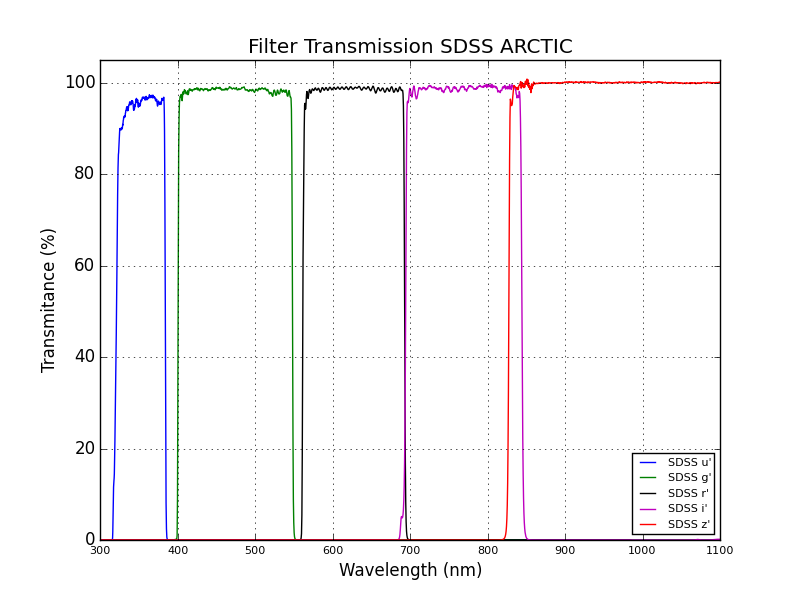
The six position filter wheel in ARCTIC can take up to 130mm round filters. We have SDSS u',g',r',i',z' and Johnson U,B,V,R,I full field filter sets. The 3" square filters used in SPIcam can be used, but require an adapter and will limit the field of view to 4.5'. The smaller 2" filters can also be used with an appropriate adapter, and will limit the field futher. Other filter sizes, up to 130mm round, can also be used with the appropriate adapter. For other The full set of filters available at APO can be found at the APO Filter Database.
Below is a plot of the SDSS filter bandpasses and transmission for the available 130mm set.
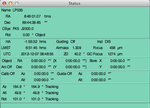
ARCTIC is operated within the Telescope User Interface (TUI) software written and maintained by Russell Owen at the University of Washington. A detailed manual is available here. The main TUI status window looks like this:
2.2. Configuring the Instrument
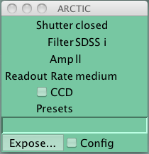
The instrument is configured using the ARCTIC window accessible under the Inst menu from the main TUI window. This brings up the ARCTIC control gui. Here we give brief overview of the ARCTIC controls via the ARCTIC control gui:
This window shows the current configuration (Shutter state, filter, binning, windowing, image size, overscan area). The configuration can be changed using the Show Config button; as with other TUI windows, the Apply button must be hit to implement any selected changes and all current selections are applied upon click.
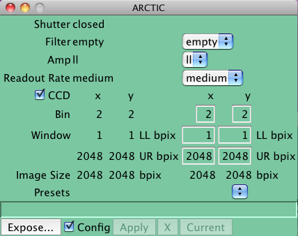
Generally, the main item that is configured is changing the filter. The CCD binning is also configurable here, but is generally set to a value at the beginning of the night, and then left unchanged. This is done by clicking the CCD button in the config window. It will look like this:
Note that it is possible to write scripts to take sequences of exposures, e.g., changing filters between each exposure. The simplest scripts are just lists of low-level ARCTIC commands, which are presented in Appendix D. More complex scripts with GUI interfaces can be written; see the TUI manual for more information.
ARCTIC exposures are taken using the Expose window which is opened using the Expose button in the ARCTIC configuration window. The expose gui looks like:
The expose window is in standard TUI format (for detailed description see here ), and, as for other instruments, shows status of the current exposure at the top, and allows you to set the object Type (for the FITS image header), exposure Time, number of Exposures, and root File Name. If you wish to add comments to the file header, place them in the Comments field.
All data will automatically be stored on arc-gateway under /export/images/<program ID>/<filename>. However, most users set TUI up to automatically transfer images to their local computer using the Preferences options in the main TUI window menu (see AutoGet and Save To options under Exposures). You can also define a subdirectory (TUI will even create it for you) by entering a name such as <subdir1>/<subdir2>/<filename> ;note, however, that a separate image number sequence will be started in each subdirectory.
The FITS header for each image stores the exposure time values (duration, start, stop) plus telescope parameters for future reference.
The Start button begins the exposure or exposure sequence.
- Start - This button starts the exposure or exposure sequence.
- Pause - This button pauses the exposure, you can start it again later.
- Stop - This button stops the exposure AND saves the current data to disk
- Abort - This button aborts an exposure. It DOES NOT save the data.
Guiding while using ARCTIC is accomplished through use of the off-axis guider on the NA2 port.Control of the NA2 guide camera is obtained via the Guide selection in the main TUI window. This will open the following GUI:
To guide, find a star located in the guide camera image and guide on it via Field Star guiding. Manual guiding does not send guide corrections to the telescope, but just continues to take images.
You can guide on any object which is symmetric (galaxies with strong cores are fine), not too faint, and non-saturated. Optical double stars, late-type galaxies, and bipolar PNs may pose a problem for guiding, as will objects where you desire to observe a position away from the bright center (e.g., SNs near bright galaxies). Any object the guide software thinks is usable will be circled in green. If your favored guide object is not circled, it may be too faint, too bright, or too lumpy. If you really want to use an object that has no circle around it, try dragging a box around it to centroid it. If this succeeds (if a circle appears) then you are all set.
Use longer exposure times to get better signal from your star. The best exposure times are 5-30 seconds, but up to 120 seconds is usable if you can be patient. Longer exposure times can also help if you're having data transfer problems. Exposures shorter than about 3s are a waste of image-transfer bandwidth and may cause you to over-guide on seeing fluctuations. See more about guiding in Guiding with TUI User's Guide.
The telescope is focused by inspection of ARCTIC images. Generally, focusing is most efficiently accomplished by letting the Observing Specialist focus the telescope. A focus script is available under the Scripts/ARCTIC/Focus TUI menu; this is what is used by the observing specialists to focus and provide a current seeing estimate.
As with all instruments, monitoring focus is advisable, as it will change over the course of the night, especially at the beginning of the night before the telescope has reached equilibrium.
Because ARCTIC is located on the NA2 image rotator, the chip can be oriented however the user prefers. At a Rot angle of 0, N is in the direction of increasing rows, and W in the direction of increasing columns.
The following table summarizes some of the chip characteristics when using the default read and binning settings of medium and 2x2; see more details in subsequent sections:
Number of rows Number of columns Pixel size Gain Readout noise Field of View 7.85 arcmin
Platescale Readout time is 25 seconds in the default medium readout mode, through amplifier II. Through the same amplifier, fast readout time is 11 seconds.
3.2. Detector Layout/Cosmetics
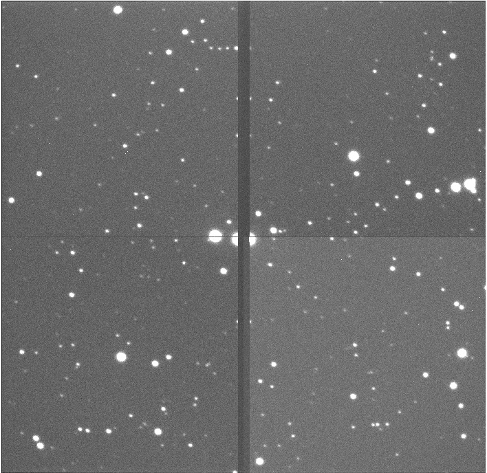
This detector is structured in four quadrants which can be read out individually or as a whole. When reading out the whole detector the user can select any of the four amplifiers (located on the corners of the chip). There are three readout modes, slow, medium, and fast, as well as three binning options in both x and y directions. Standard operating mode is medium read with 2x2 binning. There is a 100 pixel overscan area in the x direction in 1x1 binning. The detector has one bright column (1808) and one trap column (2116). There are also 3 small dimples in the center of the left edge of the chip.
The detector is made of a single monolithic piece of silicon. Although the quadrants appear to look as though it is four sections of chip what it being done is that a windowed section of the silicon is being read out through independent amplifiers. The benefit is greatly improved readout speed. When in single amplifier mode the overscan appears on the right. This should look like a normal CCD image. In quad amplifier mode the four overscan regions (one for each amplifier) is placed in the center. NOTE: the overscan in the center of the chip is NOT a physical section of the detector. An example of a quad read image in the raw form and with the ovescan removed with the quicklook software can be seen below. Notice how the star in the center was recovered. It is not recommended to place a target on different quadrants but for demonstration purposes it shows the monolithic structure of the device.
Quad Readout Raw Image Frame Quad Mode Overscan Removed
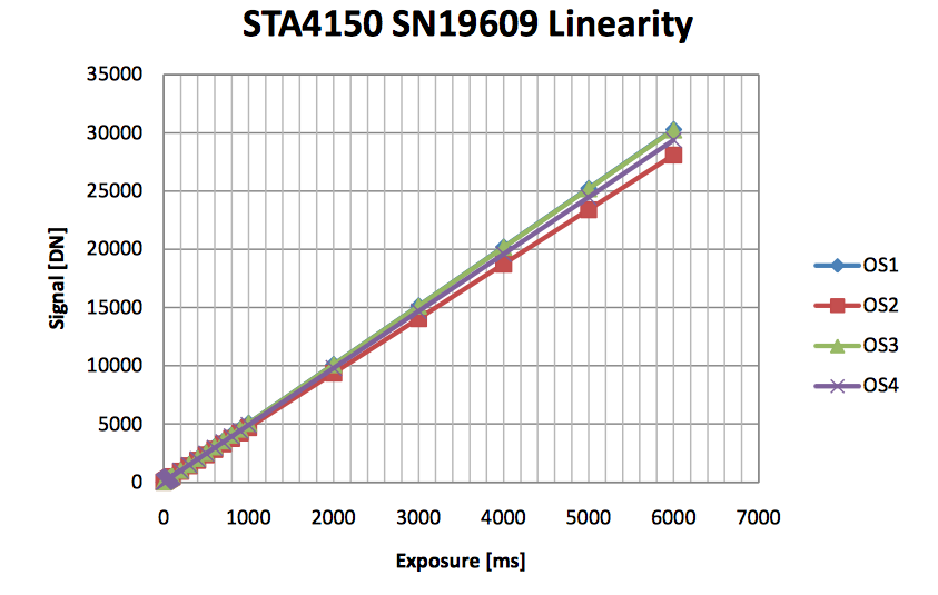
3.3. Detector Linearity/Saturation at 60000 counts
The CCD is linear (within 1%) up to saturation, i.e. the full range of the A/D converter. The following plot demonstrantes this performance. Each line (OS 1-4) represents one of the four readout amplifiers on the chip.
3.4. Detector Gain and Readout Noise
The gain has been measured to be 2.00 electrons/pixel, with a readout noise of 3.7 electrons in the medium readout mode.
NOTE--- Add matrix of gain, RN, amplifier!!
Readout Option Speed RN Slow 150 kHz 3.4 Medium 450 kHz 3.7 Fast 900 kHz 6.0 ???
Amplifier Gain Read Noise 1 --- --- 2 1.99 3.8 3 --- --- 4 --- ---
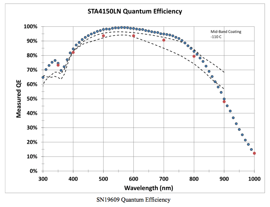
The following table and plot show the CCD quantum efficiency, as measured by ITL. The table is taken from the plot, for a quick and easy reference at specific wavelengths. In the plot, the black dashed lines are coating information used by Mike Lesser. The red dots are 1-r measurements. And the blue dots are the actual diode measurements on our chip. This is the important line, and the source for the quick look table.
Wavelength (nm) QE (%) Notes 350 75 measured 400 85 measured 500 98 measured 550 99 measured 600 98 measured 700 95 measured 800 84 measured 900 50 measured 1000 12 measured
The minimum exposure time permitted by the control software is 0.1s. Shutter timing accuracy has been tested down to 0.25s, but very short science exposures may suffer from seeing variations. Many of the most popular Landolt and SDSS standard stars will saturate in broadband filters with times as short as 1s, so it's recommended to look for standards around magnitude 13 or fainter for broadband observations, and then exposure times of 5-10s should be effective depending on waveband and atmospheric conditions.
Biases, flats, and darks are necessary for calibration. See the following sections for details.
4.1. Calibration Lamps and Control
There are bright and dim quartz lamps located on the truss at the top of the telescope that can be used for flat fields, taken off of the mirror covers. These are controlled by the Truss Lamps GUI under the Misc item in the command bar in the main TUI window. In contrast with many other TUI controls, these are turned on and off by simply hitting the On/Off buttons; there is no Apply button for these lamps.
Flat fields can be taken by shining the truss lamps onto closed primary mirror covers; no "white spot" is used at the 3.5m. Since the installation of improved baffling in the telescope, these "mirror cover" flats provide reasonable measurements of the variation in instrument/telescope response over the ARCTIC field of view. Although twilight flats are still preferable and superflats taken from object images are best of all, mirror cover flats are a desirable alternative when the other kinds are not possible. Mirror cover flats will be slightly redder than the twilight sky or the night sky, and may therefore be more appropriate for photometry of red targets through broadband filters. Another issue is that long exposures are required for the bluest filters with the current calibration lamps.
Thanks to the new baffle, the illumination pattern of mirror cover flats now has very little dependence on rotator position, except in the outer corners of the image. Observers planning aperture photometry on small objects near the center of the field should not have to worry about rotator position for mirror cover flats. Observers doing surface photometry on larger objects or aperture photometry of multiple targets throughout the field may want to take flats at multiple rotator positions and combine them into a master flat. This does require coordination with the observing specialist, since we have to be very careful about having the mirror covers closed and motors active at the same time -- so be sure to communicate your plans clearly to the observing specialist.
Here are some suggested exposure times that should give 20K-30K counts for either the SDSS or the Johnson-Cousins 5-inch round filters. We do not have a current set of exposure suggestions for narrowband filters. We also recommend doing them in this order: u', z', r', g', i' or U, B, V, Rc, Ic.
u' Brt Qtz 180s g' Dim Qtz 15s r' Dim Qtz 5s i' Dim Qtz 2s z' Dim Qtz 3.5s U Brt Qtz 70s B Brt Qtz 5s V Dim Qtz 10s Rc Dim Qtz 3s Ic Dim Qtz 2s Twilight flats are a good option for observations scheduled adjacent to twilight, and will have an illumination pattern more like science data at the edges of the image, as compared to dome flats which have additional vignetting. Narrowband filters may be ready for sky flats starting five minutes after sunset; flats in broadband filters can start about 15 minutes after sunset. Remember that the detector is linear to a high level, so sky levels between 10K to 50K counts can make good flats. The illumination pattern in the flats results from the telescope baffling, not from shutter behavior, so it's safe to take flats at a fraction of a second. If you are using a readout mode with a readout time less than 7s, you might want to stop the telescope tracking and take flats with stars trailing through the images. For readout time longer than 7s, simply make a relative offset of any size or type in between exposures to make sure that stars don't fall on the same pixels. We do not currently have a script for taking sky flats automatically.
Fringing will occur in deep exposures through the J-C R or I filters, the SDSS i or z filters, and potentially any red broadband filter. Fringe strength can very from night to night or hour to hour and may be worse for observations made in the northwestern sky (above the sodium lights of Alamogordo). The best method for removing fringes is to obtain a superflat made from data images. This may require taking multiple images of a field with dither offsets in between, or images of different fields in the same part of the sky may be combined. Some observers have also worked on creating master fringe flats which could be scaled and applied to data.
It may be necessary to throw away the first one or two bias images if the instrument was idle before taking biases. Some reduction guides on the User Wiki recommend throwing away more of the initial images, or taking frequent biases in between object exposures; that recommendation was based on behavior that occurred when the instrument's operating temperature was 155 C during the first year and a half of operation. As of January 2017, the instrument's operating temperature was raised to 186 C, which results in more stable bias behavior.
The higher operating temperature does necessitate dark frames for calibration of exposures longer than about 60s. Between 30s to 60s dark subtraction may help or may just add noise. Applying dark subtraction to exposures shorter than 30s is not recommended. The dark pattern is stable and dark current levels vary linearly with exposure time (for exposures longer than 30s), so it's advisable to take a few darks of 5 minutes or your longest science exposure time, whichever is higher, combine these to make a master dark, and then scale the master dark according to the exposure time.
The last row on the detector is always saturated. This is a feature in the controller electronics. There is a bright column (1808) and a trap column (2116)
There are three small dimples in the detector silicone. They are near the center of the left edge.
5.3. Overscan and Cosmic Ray behavior
There are some peculiarities of the different readout modes which may affect which mode is best for a particular science program. In single-readout mode (LL), the overscan does not match the bias level very well so it's very important to be sure to subtract overscan and subtract biases if you are using this mode. In quad readout mode, the overscan behavior is more consistent with the bias levels. This may make quad mode more desirable if you are doing short exposures with low background levels that are not much above the bias level.
However, quad readout move sometimes misbehaves when a cosmic ray hits the detector with enough energy to saturate at least one pixel. Rows which have a saturated cosmic ray in them (or, inconsistently, sometime a saturated star) might show a charge trail persisting across hundreds of columns, or even a step function in the bias level starting at the row of the cosmic ray. The step function can be removed by overscan subtraction, but at least one row will still show the effects. Single-readout mode does not display this behavior except for extreme saturation events. So if you are doing longer exposures with high sky levels and many cosmic rays, it may be better to use LL readout to avoid getting many trails across your images.
Be sure to turn off any calibration lamps you may have used, then hand over the instrument by simply quitting out of the ARCTIC instrument control window in TUI. In some circumstances, you may continue to use the instrument after your shift, e.g., you are the first half observer and the scheduled second-half observer is not using the ARCTIC. Ask your Observing Specialist for permission to do so if circumstances warrant.
6.1. Data Storage and Retrieval
Your data will remain on arc-gateway.apo.nmsu.edu:/export/images/your program code/UTYYMMDD/ for 9 to 12 months before being automatically deleted. Data can be accessed via scp or to the institutions' observer accounts on arc-gateway (you can also use ftp and the images account and password); call APO (575-437-6822) if you are unsure of the correct login.
Please find additional information for taking and reducing data here.
A. Instrument Design
See the ARCTIC Commissioning Report.
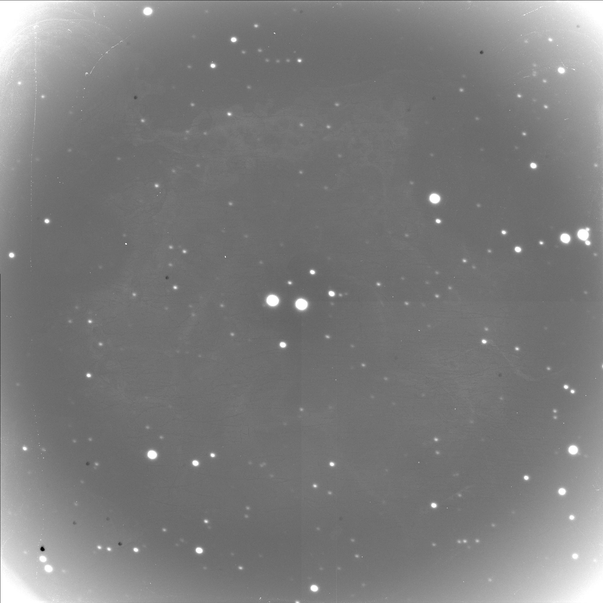
Please note that there is some vingetting toward the edges of the field, several arcminutes from center. You will notice stars get fainter closer to the edge.
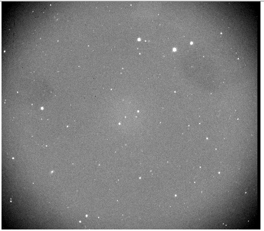
This is an example of a typical science image, using the SDSS i' filter.
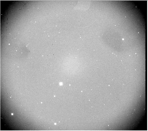
This is an example of a typical sky flat, using the SDSS i' filter.
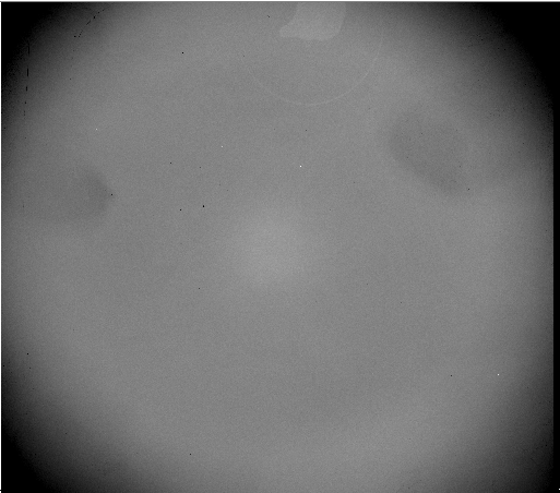
This is an example of a typical dome flat, using the SDSS i' filter.
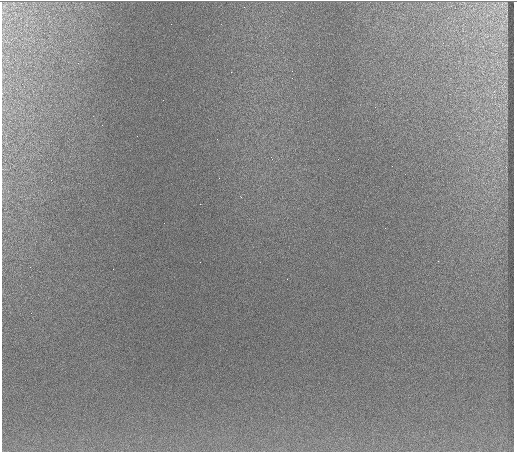
This is an example of a typical bias frame in LL readout mode. Note the disparity between bias and overscan at the right side of the chip.
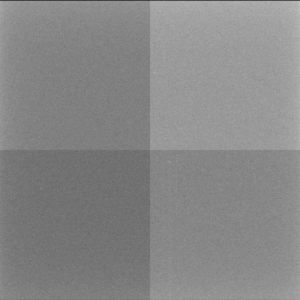
This is an example of a typical bias frame in quad readout mode. The boundaries between quadrants are visible, but the transition from bias to overscan is not.
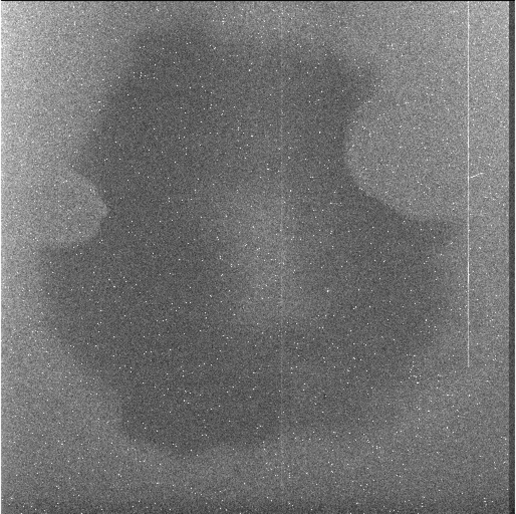
This is an example of a 5-minute dark frame in LL readout mode, at the operating temperature of 186 K in use after January 2017.
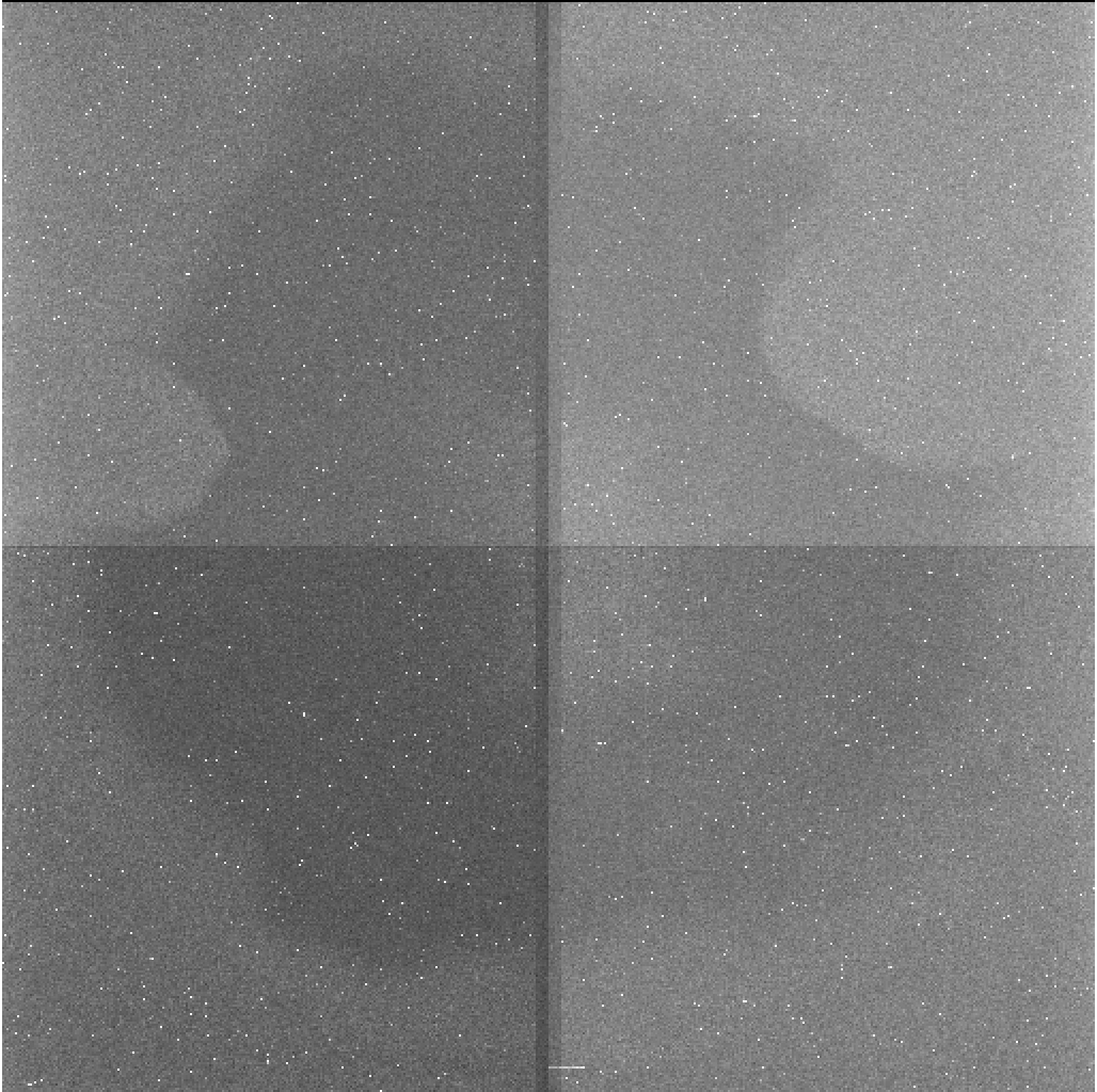
This is an example of a 5-minute dark frame in quad readout mode, at the operating temperature of 186 K in use after January 2017. A cosmic ray near the bottom of the image displays a trailing problem.
D. Basic Low-level Commands (for scripting)
arctic set filter=1|2|3|4|5|6 : sets filter to specified position
arcticExpose object|flat|dark|bias time=time [n=nexp] [name=root] : takes specified type of exposure, with specified exposure time, [number of exposures], [root file name]
Examples:
arctic set filter=1 #(this command will change the filter wheel to filter position 1)
arcticExpose object time=10 n=1 name=spicam_exposure #(this command will take 1 object image of time 10s with the name spicam_exposure.fits) If making a Run_Command script TUI knows to wait for commands to be executed before continuing so listing one command after another is acceptable.